Content

• Steps
• Part 1 of 2: Preparing the data for the chart
• Part 2 of 2: Creating a Chart
• Tips

This article will teach you how to create a visual presentation of data in Microsoft Excel using pie charts.

Steps

Part 1 of 2: Preparing the data for the chart

1. 1 Start Microsoft Excel. The program icon, depending on the version, is a green or white letter "X" on a white-green background.
   • If you need to create a chart based on the data you already have, just double-click the Excel document that contains the data to open it and skip straight to the next part of the article.
2. 2 Click on the New Workbook (on a regular PC) or Excel Workbook (on a Mac) button. It will be located at the top left of the Available Templates window.
3. 3 Enter a title for the chart. To do this, select the cell B1, and then enter a title for the future chart.
   • For example, if the chart is going to represent a budget structure, the title might be "2017 Budget".
   • You can also enter an explanation for the title in the cell A1, for example: "Budget allocation".
4. 4 Enter data for the chart. Enter the name of the sectors of the future diagram in the column A and the corresponding values ​​into the column B.
   • Continuing the example with the budget, you can specify in the cell A2 "Transportation costs", and in the cell B2 put the corresponding amount of 100,000 rubles.
   • The chart will calculate the percentages for each article listed for you.
5. 5 Finish entering data. Once you complete this process, you can start creating a chart based on your data.

Part 2 of 2: Creating a Chart

1. 1 Highlight all your data. To do this, first select the cell A1, hold down the key ⇧ Shift, and then click on the bottommost cell with data in the column B... This will highlight all of your data.
   • If your chart will use data from other columns or rows of the workbook, just remember to select all of your data from the top left corner to the bottom right corner while holding down ⇧ Shift.
2. 2 Click on the Insert tab. It's located at the top of the Excel window to the right of the home tab "the main’.
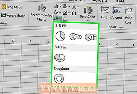
3. 3 Click on the pie chart image. This is a round button in the "Charts" button group located below and slightly to the right of the tab title "Insert". A pop-up menu will open with several options.
   • Option "Circular"allows you to create a simple pie chart with colored sectors based on your data.
   • Option "Volumetric circular"allows you to create a 3-D chart with colored sectors.
4. 4 Select the chart option you want. This step will create the chart type of your choice based on your data. Below the diagram, you will see a legend with the explanation of the corresponding diagram colors.
   • You can also use a preview of the appearance of the future diagram by simply hovering the mouse pointer over any of the proposed diagram templates.
5. 5 Customize the appearance of the chart as you wish. To do this, click on the "Constructor"at the top of the Excel window, and then navigate to the Chart Styles button group. Here you can change the appearance of the chart you create, including the color scheme, text placement, and whether percentages are displayed.
   • To make a tab appear in the menu "Constructor", the diagram should be highlighted. To select a diagram, simply click on it.

Tips

• You can copy and paste the diagram into other programs in the Microsoft Office suite (such as Word or PowerPoint).
• If you need to create charts for different datasets, repeat all steps for each of them. As soon as a new graph appears, click on it and drag it away from the center of the sheet in the Excel document so that it does not cover the first graph.