Content

• Steps
• Method 1 of 3: Conditional Formatting Option on Windows
• Method 2 of 3: Conditional Formatting Option on Mac
• Method 3 of 3: Changing the table style settings

This article will show you how to highlight every other line in Microsoft Excel on Windows and macOS computers.

Steps

Method 1 of 3: Conditional Formatting Option on Windows

1. 1 Open the spreadsheet in Excel where you want to make changes. To do this, just double-click on the file.
   • This method is suitable for all types of data. With its help, you can edit the data at your discretion, without affecting the design.
2. 2 Select the cells you want to format. Move the cursor over the desired location, press and hold the left mouse button and move the pointer to select all the cells in the range you want to format.
   • To select every second cell in the entire document, click the button Select all... It's a gray square button / cell in the upper left corner of the sheet.
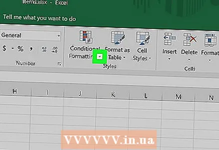3. 3 Press next to the Conditional Formatting option. This option is on the Home tab, in the toolbar at the top of the screen. A menu will appear.
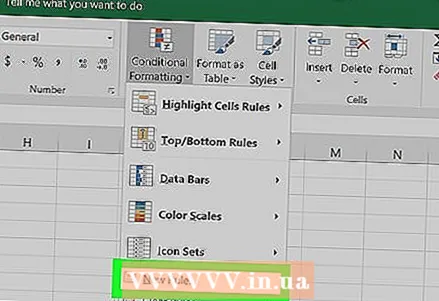4. 4 Press Create rule. The Create Formatting Rule dialog box appears.
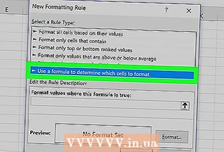5. 5 In the "Select a Rule Type" section, select Use a formula to define formatted cells.
   • If you have Excel 2003, choose Formula from the Condition 1 menu.
6. 6 Enter a formula that highlights every other line. Enter the following formula in the text area:
   • = MOD (ROW (), 2) = 0
7. 7 Click on the button Format in the dialog box.
8. 8 Open the tab Fill at the top of the dialog box.
9. 9 Select the pattern or color for the cells you want to shade and click OK. A color swatch appears below the formula.
10. 10 Click on OKto highlight every other cell on the sheet with the selected color or pattern.
    • To change the formula or format, click the arrow next to the Conditional Formatting option (on the Home tab), select Rule management, and then select a rule.

Method 2 of 3: Conditional Formatting Option on Mac

1. 1 Open the spreadsheet in Excel where you want to make changes. As a rule, it is enough to double-click on the file to do this.
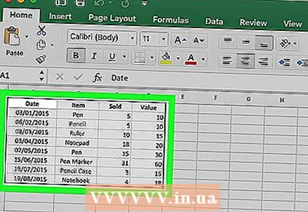2. 2 Select the cells you want to format. Move the cursor to the desired place, press the left mouse button and, while holding down, move the pointer to select all the cells in the desired range.
   • If you want to select every second cell in the entire document, press ⌘ Command+A on keyboard. This will select all the cells on the sheet.
3. 3 Press next to the Conditional Formatting option. This option is on the Home tab, in the toolbar at the top of the screen. After that, you will see several options for formatting.
4. 4 Click on the option Create rule. A new New Formatting Rule dialog box appears with several formatting options.
5. 5 From the Style menu, choose classical. Click on the Style drop-down menu and then select classical at the bottom.
6. 6 Select item Use a formula to define formatted cells. Click on the drop-down menu under the Style option and select Use formulato change the format using a formula.
7. 7 Enter a formula that highlights every other line. Click the formula box in the Create Formatting Rule window and enter the following formula:
   • = MOD (ROW (), 2) = 0
8. 8 Click on the dropdown next to the option Format with. It is located at the very bottom, under the field for entering the formula. A drop-down menu with options for formatting will appear.
   • The selected format will be applied to every second cell in the range.
9. 9 Choose a format from the Format Using drop-down menu. Select any option and then view a sample on the right side of the dialog box.
   • If you want to create a new selection format of a different color yourself, click on the option its format at the bottom. This will bring up a new window where you can manually enter fonts, borders and colors.
10. 10 Click on OKto apply formatting and highlight every other line in the selected range on the sheet.
    • This rule can be changed at any time. To do this, click on the arrow next to the "Conditional Formatting" option (on the "Home" tab), select Rule management and select a rule.

Method 3 of 3: Changing the table style settings

1. 1 Open the spreadsheet in Excel that you want to modify. To do this, just double-click on the file (Windows and Mac).
   • Use this method if, in addition to highlighting every second line, you also want to add new data to the table.
   • Use this method only if you do not want to change the data in the table after you format the style.
2. 2 Select the cells you want to add to the table. Move the cursor over the desired location, press the left mouse button and, while holding down, move the pointer to select all the cells that you want to change the format of.
3. 3 Click on the option Format as table. It is located on the "Home" tab, on the toolbar at the top of the program.
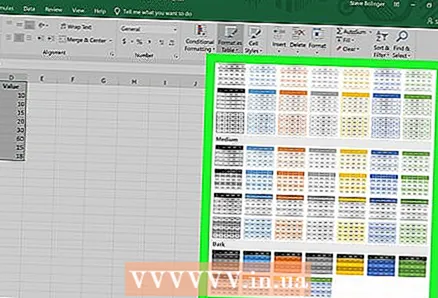4. 4 Select a table style. Browse through the options under Light, Medium, and Dark and click on the style you want to apply.
5. 5 Click on OKto apply the style to the selected data range.
   • To change the style of a table, enable or disable the options under Table Style Options in the toolbar. If this section is not there, click on any cell in the table and it will appear.
   • If you want to convert the table back to a range of cells in order to be able to edit the data, click on it to display the options in the toolbar, open the tab Constructor and click on the option Convert to Range.