Content

• Steps
• Method 1 of 2: Excel 2013
• Method 2 of 2: Excel 2010, 2007, 2003
• Tips
• Warnings

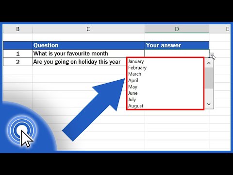
A drop-down list in Microsoft Excel can improve data entry efficiency, but at the same time restrict data entry to a specific set of items or to the data in the drop-down list.

Steps

Method 1 of 2: Excel 2013

1. 1 Open the Excel file in which you want to create the dropdown list.
2. 2 Select blank or create a new sheet.
3. 3 Enter the list of items to be displayed in the dropdown list. Each item is entered in a separate cell on each new row. For example, if you create a drop-down list with sports names, enter baseball in A1, basketball in A2, football in A3, and so on.
4. 4 Select the range of cells that contains all of the items you entered.
5. 5 Click on the "Insert" tab. Select "Name" and then select "Set".
6. 6 Enter a name for the items in the Name field and click OK. This name is for reference only and will not appear in the table.
7. 7 Click on the cell where you want to create the dropdown list.
8. 8 Click the Data tab and select Data Validation from the Data Tools group. The "Validate Input Values" window opens.
9. 9 Click the "Options" tab. Select "List" from the "Data Type" drop-down menu.
10. 10 In the line "Source" enter an equal sign and the name of your drop-down list. For example, if your dropdown is called Sports, enter = Sports.
11. 11 Check the box next to "List of acceptable values".
12. 12 Check the box next to "Ignore empty cells" if you want users to be able to select zero items from the drop-down list.
13. 13 Click the Error Message tab.
14. 14 Check the box next to "Display error message". This option prevents users from entering incorrect data.
15. 15 Click OK. The dropdown list appears in the spreadsheet.

Method 2 of 2: Excel 2010, 2007, 2003

1. 1 Open the Excel file in which you want to create the dropdown list.
2. 2 Select blank or create a new sheet.
3. 3 Enter the list of items to be displayed in the dropdown list. Each item is entered in a separate cell on each new row. For example, if you are creating a drop-down list with the names of fruits, enter "apple" in cell A1, "banana" in cell A2, "blueberries" in cell A3, and so on.
4. 4 Select the range of cells that contains all of the items you entered.
5. 5 Click in the Name box to the left of the formula bar.
6. 6 In the Name field, enter a name for the drop-down list that describes the items you entered, and then press Enter. This name is for reference only and will not appear in the table.
7. 7 Click on the cell where you want to create the dropdown list.
8. 8 Click the Data tab and select Data Validation from the Data Tools group. The "Validate Input Values" window opens.
9. 9 Click the "Options" tab.
10. 10 Select "List" from the "Data Type" drop-down menu.
11. 11 In the line "Source" enter an equal sign and the name of your drop-down list. For example, if your dropdown is called "Fruit", enter "= Fruit".
12. 12 Check the box next to "List of acceptable values".
13. 13 Check the box next to "Ignore empty cells" if you want users to be able to select zero items from the drop-down list.
14. 14 Click the Error Message tab.
15. 15 Check the box next to "Display error message". This option prevents users from entering incorrect data.
16. 16 Click OK. The dropdown list appears in the spreadsheet.

Tips

• Enter the items in the order you want them to appear in the dropdown list. For example, enter items alphabetically to make the list more user-friendly.
• After you finish creating the dropdown, open it to ensure that all of the items you entered are present. In some cases, you will need to expand the cell in order to display all the elements correctly.

Warnings

• You will not be able to access the Data Validation menu if your spreadsheet is secured or shared with other users. In these cases, remove protection or disallow sharing of this table.