Content

• Method 2 of 3: How to display a specific string
• Method 3 of 3: How to change the row height

1 Open an Excel spreadsheet. Double click on the desired Excel file to open it in Excel.

2 Click Select All. This triangular button is in the upper left corner of the table above the row 1 and to the left of the column header A... The entire contents of the table will be highlighted.

• Alternatively, you can click any cell in the table and then click Ctrl+A (Windows) or ⌘ Command+A (Mac) to select all table contents.

3 Click on the tab the main. It's at the top of the Excel window.

• If you are already on the Home tab, skip this step.

4 Click on Format. It's under the Cells section of the toolbar. A menu will open.

5 Please select Hide or show. This option is located in the Format menu. A pop-up menu will appear.

6 Click on Display lines. This option is on the menu. All hidden rows are displayed in the table.

• To save your changes, click Ctrl+S (Windows) or ⌘ Command+S (Mac).

Method 2 of 3: How to display a specific string

1. 1 Open an Excel spreadsheet. Double click on the desired Excel file to open it in Excel.
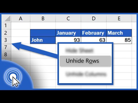
2. 2 Find the hidden line. Look at the line numbers on the left side of the table; if some number is missing (for example, after the line 23 there is a line 25), the line is hidden (in our example, between the lines 23 and 25 hidden line 24). You will also see a double line between the two line numbers.
3. 3 Right click on the space between the two line numbers. A menu will open.
   • For example, if the line is hidden 24, right click between numbers 23 and 25.
   • On a Mac computer, click Control and click on the space to open the menu.
4. 4 Click on Display. This option is on the menu. This will display the hidden row.
   • To save your changes, click Ctrl+S (Windows) or ⌘ Command+S (Mac).
5. 5 Display a series of lines. If you notice that there are multiple lines hidden, display them by following these steps:
   • hold Ctrl (Windows) or ⌘ Command (Mac) and click on the line number above the hidden lines and on the line number below the hidden lines;
   • right-click on one of the selected line numbers;
   • select "Display" from the menu.

Method 3 of 3: How to change the row height

1. 1 Know when to use this method. You can hide a row by decreasing its height. To display such a row, set the value to "15" for the height of all rows in the table.
2. 2 Open an Excel spreadsheet. Double click on the desired Excel file to open it in Excel.
3. 3 Click Select All. This triangular button is in the upper left corner of the table above the row 1 and to the left of the column header A... The entire contents of the table will be highlighted.
   • Alternatively, you can click any cell in the table and then click Ctrl+A (Windows) or ⌘ Command+A (Mac) to select all table contents.
4. 4 Click on the tab the main. It's at the top of the Excel window.
   • If you are already on the Home tab, skip this step.
5. 5 Click on Format. It's under the Cells section of the toolbar. A menu will open.
6. 6 Please select Line height. This option is on the menu. A pop-up window will open with an empty text box.
7. 7 Enter the line height. Enter 15 in the text box of the popup.
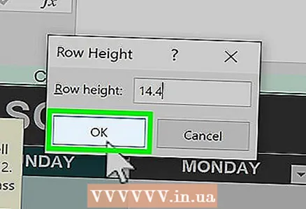8. 8 Click on OK. The height of all lines will change, including lines that have been hidden by decreasing the height.
   • To save your changes, click Ctrl+S (Windows) or ⌘ Command+S (Mac).