Content

• Steps
• Method 1 of 3: Cropping Text Using LEFT and RIGHT (English LEFT and RIGHT)
• Method 2 of 3: Cropping Text Using MID (MID English)
• Method 3 of 3: Splitting Text into Multiple Columns
• Additional articles

This article will teach you how to crop text in Microsoft Excel. To do this, you first need to enter the complete, non-truncated data into Excel.

Steps

Method 1 of 3: Cropping Text Using LEFT and RIGHT (English LEFT and RIGHT)

1. 1 Start Microsoft Excel. If you have already created a document with data that requires processing, double-click on it to open it. Otherwise, you need to start Microsoft Excel to create a new workbook and enter data into it.
2. 2 Select the cell in which the shortened text should be displayed. This must be done when you have already entered raw data into the workbook.
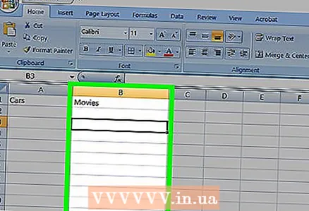
   • Note that the selected cell must be different from the cell that contains the full text.
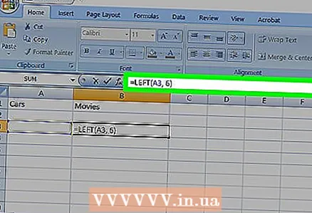3. 3 Enter the formula LEFT or RIGHT in the highlighted cell. The principle of operation of the LEFT and RIGHT formulas is the same, despite the fact that LEFT reflects a given number of characters from the beginning of the text of a given cell, and RIGHT - from its end. The formula you enter should look like this: "= LEFT (cell address with text; number of characters to display)". You do not need to enter quotation marks. Below are some examples of the use of the mentioned functions.
   • Formula = LEFT (A3,6) will show the first six characters of the text from cell A3. If the original cell contains the phrase "cats are better", then the truncated phrase "cats" will appear in the cell with the formula.
   • Formula = RIGHT (B2,5) will show the last five characters of the text from cell B2. If cell B2 contains the phrase "I love wikiHow", then the truncated text "kiHow" appears in the cell with the formula.
   • Remember that spaces in the text also count as a character.
4. 4 When you are finished entering the formula parameters, press the Enter key on your keyboard. The formula cell will automatically reflect the clipped text.

Method 2 of 3: Cropping Text Using MID (MID English)

1. 1 Select the cell where you want the clipped text to appear. This cell must be different from the cell that contains the processed text.
   • If you have not yet entered the data for processing, then this must be done first.
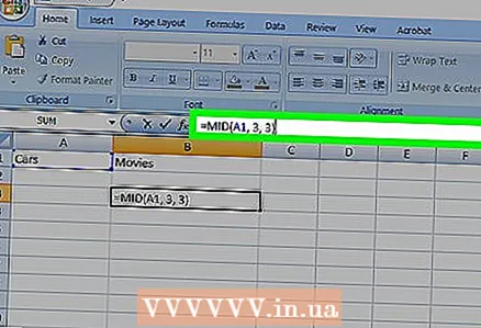2. 2 Enter the MID formula in the highlighted cell. The MID function allows you to extract text from the middle of a line. The entered formula should look like this: "= PSTR (address of the cell with the text, the ordinal number of the initial character of the extracted text, the number of characters to be extracted)". You do not need to enter quotation marks. Below are some examples.
   • Formula = MID (A1; 3; 3) reflects three characters from cell A1, the first of which takes the third position from the beginning of the full text. If cell A1 contains the phrase "racing car", then the abbreviated text "night" appears in the cell with the formula.
   • Similarly, the formula = MID (B3,4,8) reflects eight characters from cell B3, starting at the fourth position from the beginning of the text. If cell B3 contains the phrase "bananas are not people", then the abbreviated text "any - not" will appear in the cell with the formula.
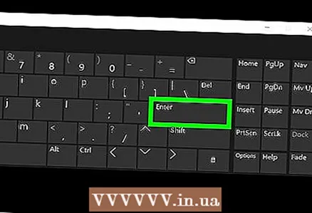3. 3 When you are finished entering the formula parameters, press the Enter key on your keyboard. The formula cell will automatically reflect the clipped text.

Method 3 of 3: Splitting Text into Multiple Columns

1. 1 Select the cell with the text you want to split. It must contain more text characters than spaces.
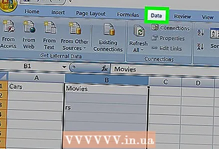2. 2 Click on the Data tab. It is located at the top of the toolbar.
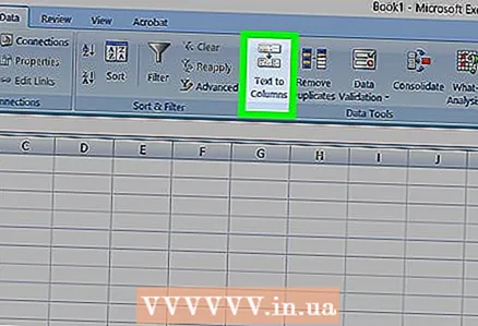3. 3 Click the Text by Columns button. This button is located on the toolbar in a group of buttons called Data Tools.
   • Using the functionality of this button, you can divide the contents of an Excel cell into several separate columns.
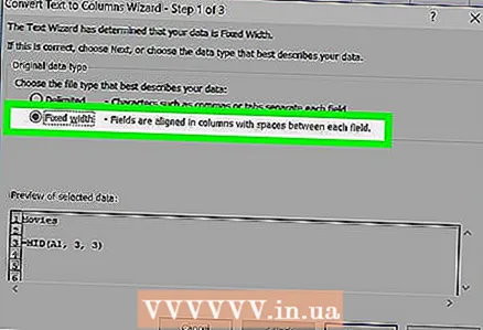4. 4 In the settings window that appears, activate the fixed width option. After clicking the Text by Columns button at the previous step, a settings window with the name "Text wizard (parsing) - step 1 of 3" will open. In the window, you will be able to choose one of two options: "delimited" or "fixed width".The "delimited" option means that the text will be delimited by spaces or commas. This option is usually useful when processing data imported from other applications and databases. The "fixed width" option allows you to create columns from the text with a specified number of text characters.
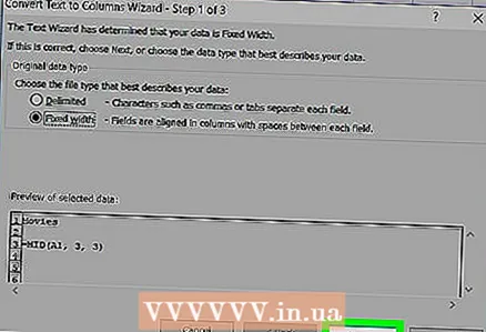5. 5 Click "Next. You will be presented with a description of three possible courses of action. To insert the end of a line of text, click at the desired position. To remove the end of a line, double-click on the dividing line. To move the end of a line, click on the dividing line and drag it to the desired location.
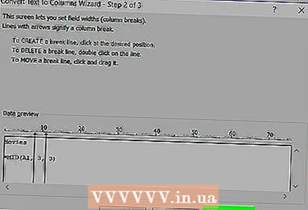6. 6 Click Next again. In this window, you will also be offered several options for the column data format to choose from: "general", "text", "date" and "skip column". Just skip this page unless you want to intentionally change the original format of your data.
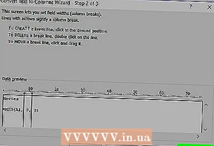7. 7 Click on the Finish button. The original text will now be split into two or more separate cells.

Additional articles

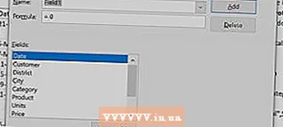How to add a column to a Pivot Table 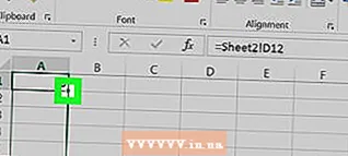How to link sheets in Excel How to sort cells alphabetically in Excel How to convert a text file (TXT) to an Excel file (XLSX) How to add a new tab in Excel How to add a second Y axis to a graph in Microsoft Excel 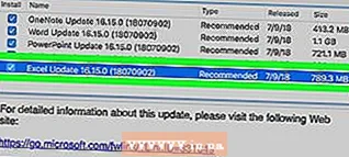How to update Excel How to calculate standard deviation in Excell How to rename columns in Google Sheets (Windows and Mac) 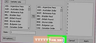How to create a currency converter in Excel How to add data to MS Excel pivot table How to change the date format in Microsoft Excel How to create a family tree in Excel How to create a pivot table in Excel