Content

• To step
• Method 1 of 3: Hyphenate text using LEFT and RIGHT functions
• Method 2 of 3: Hyphenate text with the SHARE function
• Method 3 of 3: Divide text across multiple columns

This wikiHow teaches you how to trim data in Microsoft Excel. To do this, you must first enter the unabridged data in Excel.

To step

Method 1 of 3: Hyphenate text using LEFT and RIGHT functions

1. Open Microsoft Excel. If you have an existing document where data has already been entered, you can double-click it to open it. If not, you will need to open a new workbook and enter your data there.
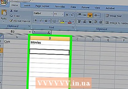2. Select the cell where you want the short version to appear. This method is useful for text you already have in your spreadsheet.
   • Note that this cell must be different from the cell in which the target text appears.
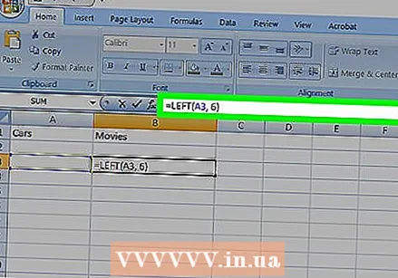3. Type the LEFT or RIGHT function in the selected cell. The LEFT and RIGHT functions use the same premise, although the LEFT function shows the characters to the left of the text in the cell and the RIGHT function shows the characters on the right. The function is "= DIRECTION (Cell name, Number of characters to display)", without the quotes. For instance:
   • = LEFT (A3, 6) shows the first six characters in cell A3. If the text in A3 says "Cats are better", then the shortened text is "Cats a" in the selected cell.
   • = RIGHT (B2, 5) shows the last five characters in cell B2. If the text in B2 says, "I love wikiHow", then the abbreviated version is "kiHow" in the selected cell.
   • Keep in mind that spaces count as characters.
4. Press Enter after entering the function. The selected cell will be automatically filled with the abbreviated text.

Method 2 of 3: Hyphenate text with the SHARE function

1. Select the cell where the truncated text should appear. This cell must be different from the cell containing the target text.
   • If you have not yet entered your data in Excel, you must do so first.
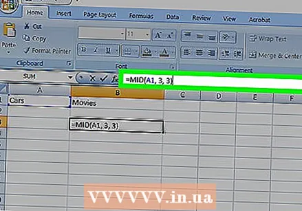2. Type the SHARE function in your selected cell. MID truncates a string in a specified cell at the beginning and end. To set the DIVIDE function, type "= DIV (Cell name, First character, Number of characters to display)" without the quotes. For instance:
   • = PART (A1, 3, 3) displays three characters from cell A1, the first of which is the third character from the left in the text. If A1 contains the text "rarity", then you will see the truncated text "rit" in the selected cell.
   • = DIVISION (B3, 4, 8) displays eight characters from cell B3, starting with the fourth character from the left. If B3 contains the text "bananas are not people", then the truncated text "an and they" will appear in your selected cell.
3. Press Enter when you are done entering the function. This will add the truncated text to the selected cell.

Method 3 of 3: Divide text across multiple columns

1. Select the cell you want to divide. This should be a cell with more characters than there is space.
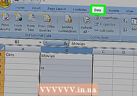2. Click on Data. This option can be found in the main menu of Excel.
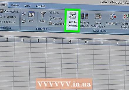3. Select Text to Columns. You can find this option in the "Data Tools" group of the Data tab.
   • This function divides the contents of the cell into multiple columns.
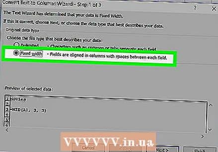4. Select Fixed width. After you press Text to columns clicked, a window will appear called "Text to Columns Wizard - Step 1 of 3". This window has two selections: "Separated" and "Fixed Width". Delimited means that characters, such as tabs or commas, will divide each field. You usually opt for separate when you import data from another application, such as a database. The "Fixed width" option means that the fields are aligned in columns with spaces between the fields.
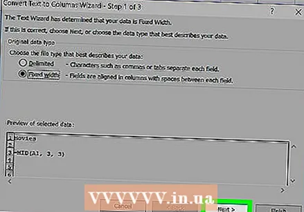5. Click on Next. This window shows three options. If you want to make a column break, click on the position where the text should be broken. If you want to delete the column break, double-click on the line. To move the line, click on it and drag the line to a desired location.
6. Click on Next again. This window has several options: "Default", "Text," "Date" and "Skip column when importing". Unless you want to force the cell formatting to be different from the default data type, you can skip this page.
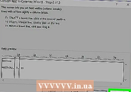7. Click on Finish. The text should now be divided into two or more cells.