Content

• Steps
• Part 1 of 3: How to enter data
• Part 2 of 3: How to Create a Graph
• Part 3 of 3: How to Choose a Graph Type

In a Microsoft Excel spreadsheet, you can build a chart or graph from the selected data. In this article, we are going to show you how to create a graph in Excel 2010.

Steps

Part 1 of 3: How to enter data

1. 1 Start Excel 2010.
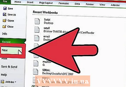2. 2 Click on the File menu to open a prepared spreadsheet or create a new one.
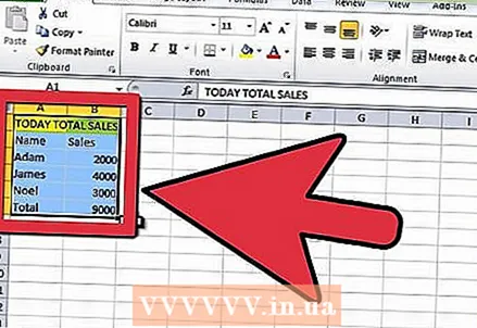
3. 3 Enter data. This is done in a certain way. Typically, names (items, products, and the like), names or dates are entered in the first column (column A), and numbers in the following columns.
   • For example, if you want to compare sales results for employees in a company, enter employee names in column A, and enter their weekly, quarterly, and annual sales results in the following columns.
   • Note that in most graphs and charts, the information in column A will be displayed on the x-axis (horizontal axis). However, in the case of a histogram, data from any column is automatically displayed on the Y-axis (vertical axis).
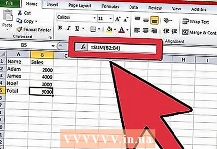4. 4 Use formulas. For example, add the data in the last cell of a column and / or row. This is necessary if you want to plot a pie chart with percentages.
   • To enter a formula, select the data in a column or row, press the fx button, and select the formula.
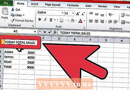5. 5 Enter a title for the spreadsheet / graph. Do it in the first lines. Use headings in the second row and column to clarify the data.
   • The titles will be transferred to the chart.
   • Data and titles can be entered in any section of the spreadsheet. If this is your first time creating a graph, try to keep the data in specific cells so that it will be easier to work with.
6. 6 Save the spreadsheet.

Part 2 of 3: How to Create a Graph

1. 1 Highlight the entered data. Hold down the mouse button and drag from the top-left cell (with the title) to the bottom-right cell (with the data).
   • To plot a simple graph from one dataset, highlight the information in the first and second columns.
   • To plot a graph based on multiple datasets, select multiple data columns.
   • Be sure to highlight the headings.
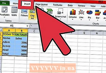2. 2 Click the Insert tab at the top of the window. In Excel 2010, this tab is located between the Home and Page Layout tabs.
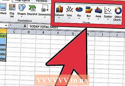3. 3 Find the "Chart" section. Various types of charts and graphs are available in this section that are used to visually represent the data in a spreadsheet.
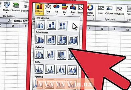4. 4 Select the type of graph or chart. Each type is marked with an icon that shows the appearance of the chart / graph.
   • To select a different type of chart, go to the "Insert" tab again and click on the icon of the desired chart in the "Chart" section.
5. 5 Hover your mouse over the graph. Right-click and choose Format Chart Area from the menu.
   • Review the options in the left pane such as Fill, Border, Drop Shadow, and so on.
   • Change the appearance of your chart / graph by choosing the colors and shadows you want.

Part 3 of 3: How to Choose a Graph Type

1. 1 Create a histogram when you are comparing multiple related items that contain multiple variables. Columns of a histogram can be grouped or stacked on top of each other (depending on how you want to compare the variables).
   • The data of one element of the table corresponds to one column of the histogram. There are no lines connecting the columns.
   • In our example with sales results, each employee will have a bar chart of a certain color. Columns of the histogram can be grouped or positioned on top of each other.
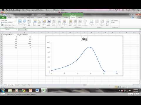
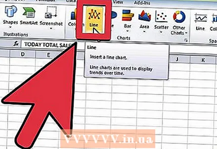2. 2 Create a line graph. It is great for showing how data changes over time (over days, weeks, or years).
   • Here one number will correspond to a point on the graph. The points will be connected with a line to show the change.
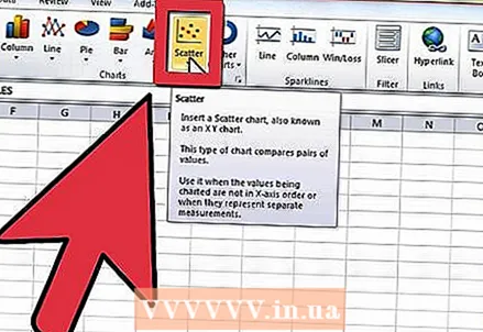3. 3 Build a scatter plot. It is similar to a line chart because data is also plotted along the X and Y axes. The points on this chart can be left as they are, or you can connect them with lines.
   • A scatter plot is great for visualizing multiple datasets where curves and straight lines may intersect. It is easy to see trends in the data in this graph.
4. 4 Select a chart type. A 3-D chart is suitable for comparing 2 datasets, a 2-D chart can show the change in value, and a Pie chart can show the data as a percentage.