Content

• Steps
• Tips

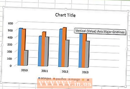
Microsoft Excel is a powerful spreadsheet editor that allows users to efficiently manage data and perform complex calculations using tables, functions and graphs. A graph (or chart) in Excel allows users to visualize numerical data and track some trend. Graphical data is much easier to understand for non-accounting staff.

Steps

1. 1 Click on the graph you want to add a title to. The highlighted graph has a thick border.
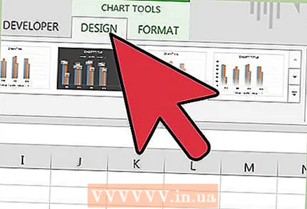2. 2 When a chart is selected, several additional tabs appear on the menu ribbon: "Constructor" and "Format". The new tabs are located in the Chart Tools tab group.
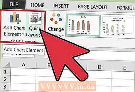3. 3 Click the Design tab and find the Chart Layouts group.
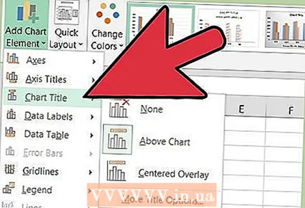4. 4 Click Add Chart Element and select Chart Title from the menu.
   • The "Center (Overlay)" option will place the title above the graph without changing its size.
   • The "Above Chart" option will place the title above the chart, but its size will be reduced.
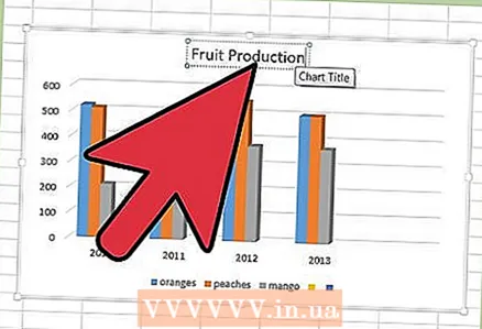5. 5 Click inside the "Chart Title" field and enter the title you want.
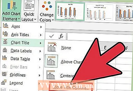6. 6 Click Add Chart Element - Chart Title - Additional Title Options.
   • Here you can change the parameters of the title, for example, add borders, fill, shadow, etc.
   • Here you can also change the parameters of the text, for example, set its alignment, direction, etc.
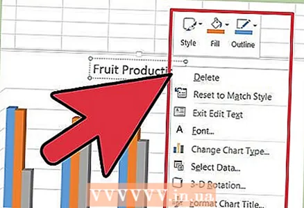7. 7 Change the font and character spacing by right-clicking on the name and choosing Font from the menu.
   • You can change the font style, size and color.
   • You can also add many different effects like strikethrough, superscript, subscript, etc.
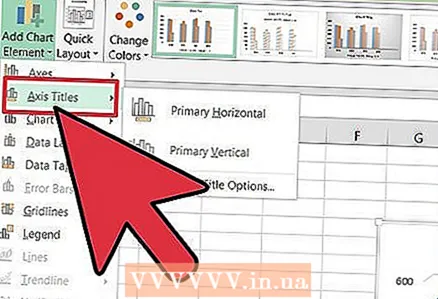8. 8 Click Add Chart Element - Axis Title to add the axis titles.
   • The Primary Horizontal option will display the name of the horizontal axis (below it).
   • The Main Vertical option will display the name of the vertical axis (to the left of it).

Tips

• You can access many of the title options simply by right-clicking on it.
• You can bind the title of a chart or axes to a specific cell in a table. Click on a title to highlight it. Then in the formula bar, enter "=" (without quotes), click on the desired cell and press Enter. Now, when information in a cell changes, the title of the chart (or axes) automatically changes accordingly.