Author:
Robert Simon
Date Of Creation:
16 June 2021
Update Date:
1 July 2024

Content
It is not difficult to copy formulas between rows and columns in Excel. However, you won't always get the results you want. In that case, or when you get #REF and / or DIV0 errors, you'll have to read more about absolute and relative references to determine where you went wrong. Fortunately, you won't have to adjust each cell in your 5,000-line spreadsheet one by one to be able to copy and paste it again. There are easy ways to automatically update formulas based on their position or copy them exactly without having to change any values.
Steps
Method 1 of 4: Drag to copy the formula to multiple cells
Enter the formula in one cell. Any formula starts with a sign = then the function or algorithm you want to use. Here, we will use a simple spreadsheet as an example and proceed to add columns A and B together: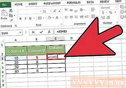
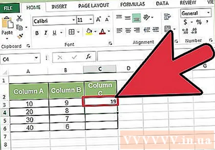
Press enter to calculate the formula. When you press the enter key, the formula will be entered and calculated. Although only the final result (19) is displayed, in fact, the spreadsheet still holds your formula.
Click the lower right corner of the original cell. Move the mouse pointer to the lower-right corner of the cell you just edited. The cursor will turn into a sign + bold.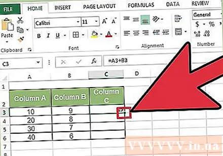
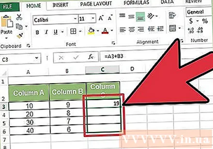
Hold down and drag the mouse along the column or row where you want to copy the formula from the original cell. Hold down the computer mouse button and drag the cursor down, down the column or horizontally, in the row where you want to edit the formula (highlighted area). The formula you entered earlier will be entered automatically in the cells you just highlighted. Relative cell references update automatically based on cells that have the same relative position. The formula used and the results displayed in our example spreadsheet will look like this: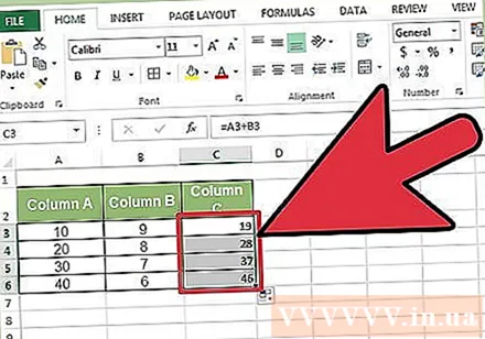
Double-click the plus sign to fill the formula out of the column. Instead of holding the mouse and dragging, you can move the mouse to the lower right corner and double-click when the pointer turns into a sign +. At this point, the formula will automatically be copied to all cells in the column.- Excel will stop filling out a column when it encounters a blank cell. Therefore, when there is a space in the reference data, you will have to repeat this step to continue filling the column section below the space.
Method 2 of 4: Paste to copy the formula into multiple cells
Enter the formula in one cell. For any formula, you need to start with a sign = then use the desired function or algorithm. Here, we will take a simple example spreadsheet and proceed to add two columns A and B together:
Press enter to calculate the formula. When you press the enter key, the formula will be entered and calculated. Even though only the results are displayed (19), the spreadsheet still preserves your formulas.- Click and copy the cell containing the original formula (CTRL + C).
- Select the cells where you want to copy the above formula. Click on a cell and use the mouse or arrow keys to drag up / down. Unlike the corner drag method, the cells where you want to copy the formula don't need to be near the original cell.
- Paste (CTRL + V). advertisement
Method 3 of 4: Copy the formula correctly
You can use this method to quickly copy a formula without having to change cell references. Sometimes, your large spreadsheet is filled with formulas, and you just want to copy them exactly. Converting everything to absolute cell references (described in the section on cell references) is not that fun, especially when you have to switch back to it after you're done. Use this method to quickly switch formulas that use relative cell references elsewhere without changing the references. In our example spreadsheet, column C needs to be copied to column D: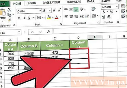
- If you only want to copy the formula in one cell, go to the last step ("Try different methods") of this section.
Opens the Find window. In most versions of Excel, you can find it by clicking the Home tab at the top of the Excel window and then clicking the Find & Select item in the "Editing" section of the Excel window. that card. You can also use the CTRL F keyboard shortcut.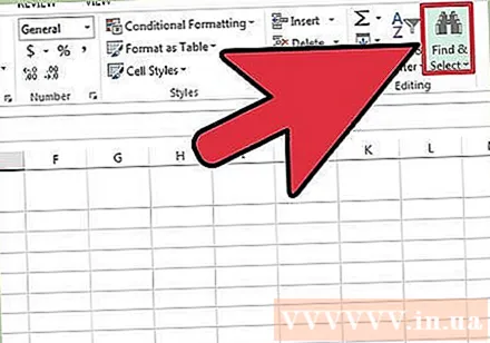
Find and replace the "=" sign with another character. Enter "=", click "Find All" then enter another character in the "Replace with" box. Any formula (always beginning with an = sign) will automatically be converted to a string of characters beginning with a certain character. Let's always use characters that are not already in your spreadsheet. For example, replace it with # or &, or a longer string, like ## &.
- Don't use * or? because they will make the following steps more difficult.
Copy and paste cells. At this point, you can select any cells you want to copy over and paste them elsewhere. Since it is no longer understood by Excel as formulas, you can now precisely copy the above cells.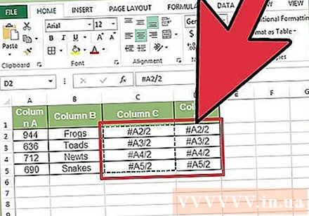
Use the Find & Replace feature again to change it back. Now that you have the recipe where you want it, you can now use "Find all" and "Replace with" to reverse it. In our example spreadsheet we will find the string "## &", replace it with an "=" sign so that the cells are formulas again and can continue editing the spreadsheet as usual:
Try other methods. If for some reason, the above method doesn't work or if you are concerned that other content in the cell might accidentally be changed by the "Replace all" option, there are a few other ways for you: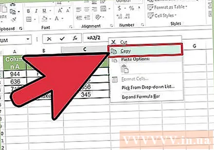
- To copy a cell's formula without changing its references, select the cell, copy the formula displayed in the formula bar near the top of the window (not the cell itself). Press esc to close the formula bar, and then paste the formula wherever you want it to be.
- Press Ctrl` (usually on the same key as ~) to switch the spreadsheet into formula view. Copy the formulas and paste them into a text editor like Notepad or TextEdit. Copy it again and paste it back into the desired location in the worksheet. Press Ctrl` to switch back to normal view.
Method 4 of 4: Use absolute and relative cell references
Use relative cell references in a formula. In an Excel formula, "cell reference" is the address of a cell. You can type or click the cell you want to use when entering the formula. In the spreadsheet below, the formula refers to cell A2: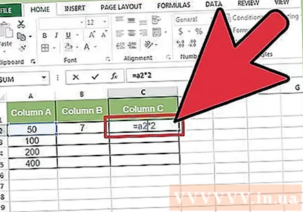
Understand why they are called relative references. In an Excel formula, a relative reference uses the relative position of a cell address. For example, cell C2 has the formula "= A2", which is a relative reference to the value of the cell to the left, one cell away. If you copy this formula to C4 it will still refer to the left cell, one cell away: now "= A4".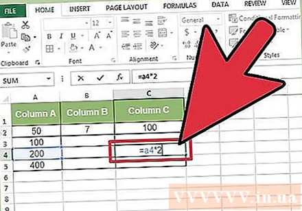
- Relative references also work for cells that are not in the same row and column. When you copy the same formula in cell C1 into cell D6 (not in the picture), Excel changes the reference one column right (C → D) and five rows down (2 → 7), and "A2" to "B7. ".
You can also use absolute references. Suppose you are not wants Excel to change its formula automatically. Then, instead of using a relative cell reference, you can convert it to a reference absolute by adding a $ symbol in front of the number of columns or rows that you want to keep when copied to any location. In the example spreadsheets below, the original formula is represented in a large, bold font, and at the same time the result of copying-pasting to other cells is displayed: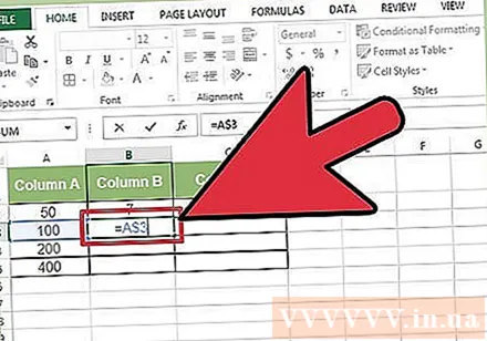
Use the key F4 to convert between absolute and relative. Click to highlight cell references in the formula. Next, press the F4 key and the $ symbol will automatically be added or removed in your reference. Keep pressing F4 until the absolute / relative reference you want appears and press enter. advertisement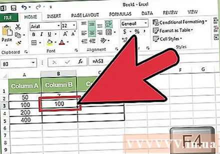
Advice
- If a blue triangle appears when you copy a formula to a new cell, Excel has detected a suspicious error. Please check the formula carefully to identify the problem.
- If you accidentally replace the = character with? or * in the method "exactly copy the formula", finding "?" or " *" will not get you the results you expected. Please fix this by searching "~?" or "~ *" instead of "?" / " *".
- Select a cell and press Ctrl (apostrophe) to copy the formula of the cell directly above it.
Warning
- Other versions of Excel may not look exactly like the screenshots in this article.


