Author:
John Stephens
Date Of Creation:
27 January 2021
Update Date:
1 July 2024

- For example, if the line 24 hidden, you will click on the space between the number 23 and 25.
- On a Mac, you can press the key Control while clicking on this space to open the menu.

Click Unhide (Unhide). This is an option in the currently displayed menu. This will make the hidden line reappear.
- You can save your changes by pressing Ctrl+S (on Windows) or ⌘ Command+S (on Mac).

Unhide many contiguous lines. If you notice many hidden lines, unhide them all with the following:
- Press Ctrl (on Windows) or ⌘ Command (on Mac) while you click on the lines above and below the lines that are hidden.
- Right-click on one of the selected lines.
- Click Unhide (Unhide) in the currently displayed menu.
Method 2 of 3: Unhide all hidden lines

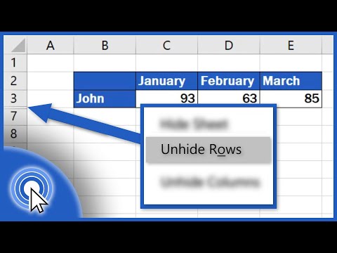
Click the "Select All" button. This rectangular button appears in the upper-left corner of the worksheet, just above the line of numbers 1 and to the left of the column header A. This is the action to select the entire Excel worksheet.- You can also click on any line in the text and press Ctrl+A (on Windows) or ⌘ Command+A (on Mac) to select the entire sheet.
Choose Hide & Unhide (Hide and unhide). This option is available from the menu Format. You will see another menu showing after the click.
Click Unhide Rows (Unhide lines). This is an option from the menu. This will immediately make hidden rows visible on the worksheet.
- You can save your changes by pressing Ctrl+S (on Windows) or ⌘ Command+S (on Mac).
Method 3 of 3: Adjusting the line heights
Click the "Select All" button. This is the rectangular button in the upper left corner of the worksheet, just above the line of numbers 1 and to the left of the column header A. This will select the entire Excel worksheet.
- You can also click any line in the worksheet and press Ctrl+A (on Windows) or ⌘ Command+A (on Mac) to select the entire sheet.
Click the card Home. This is the tab below the green section at the top of the Excel window.
- If you have already opened the card Home, please skip this step.
Click Format (Format). This is selected in the "Cells" section of the toolbar near the top-right corner of the Excel window. Another menu will appear here.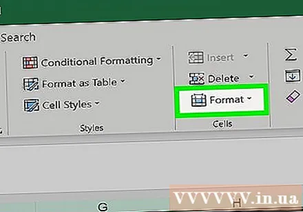
Click Row Height ... (Line height ...). This option is available from the currently displayed menu. You should see a new window appear with blank text input.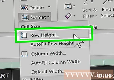
Enter the default line height. Please enter 14.4 into the text input field of the currently displayed window.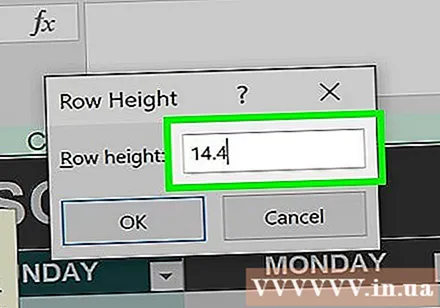

Click OK. This applies the changes to entire rows on the worksheet, and unhides rows that have been "hidden" through adjusting the line heights.- You can save your changes by pressing Ctrl+S (on Windows) or ⌘ Command+S (on Mac).


