Content

• To step
• Part 1 of 8: Making a table
• Part 2 of 8: Enlarging and reducing the table
• Part 3 of 8: Inserting and removing table rows and columns
• Part 4 of 8: Sorting table rows
• Part 5 of 8: Filtering data in tables
• Part 6 of 8: Adding a Totals row to a table
• Part 7 of 8: Add a calculation column to a table
• Part 8 of 8: Changing the style of the table
• Tips

In addition to the usual possibilities as a spreadsheet, Microsoft Excel also offers the possibility to create tables within a spreadsheet. These were called “lists” or lists in Excel 2003, and can be managed independently of the data on that worksheet or any data elsewhere in the spreadsheet. See Step 1 below for instructions on how to create and edit tables in Microsoft Excel.

To step

Part 1 of 8: Making a table

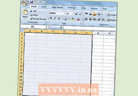1. Select a range of cells. The cells can contain data, but can also be empty, or both. If you are not sure, you do not have to select cells before creating the table.
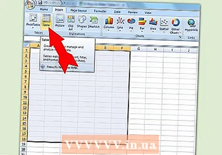2. Insert the table. To start creating the table, you will first need to insert a table into the spreadsheet.
   • In Excel 2003, click the Data menu and select List.
   • In Excel 2007, 2010 and 2013, select either "Table" from the Insert menu in the ribbon, or "Format as Table" from the Styles group in Home (Start) . The first option has to do with the default style of an Excel table, while the other allows you to choose a style while creating a table. You can later change the style of your table by choosing one of the options from the group of styles in Table Tools Design.
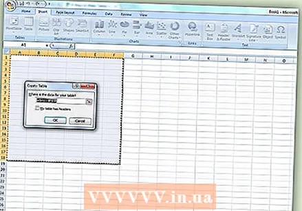3. Make sure your table has a data source. If you have not selected a group of cells at an earlier stage, it is necessary to do so now. After choosing the range, a dialog box appears, either Create Table - Create List dialog in Excel 2003 or Format As Table.
   • The field "Where is the data for your table?" (Where is the data for the table) Displays the absolute reference for the currently selected cells. If you want to change this information, you can enter other cells or a different range.
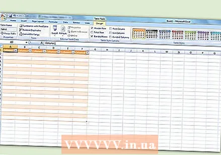4. Indicate whether your tables also have headers. If your table has headers, check the box "My table has headers". If you don't check this, the table will show the default header names ("Column 1," "Column 2," etc.).
   • You can rename a column by selecting the header and typing a name in the formula bar.

Part 2 of 8: Enlarging and reducing the table

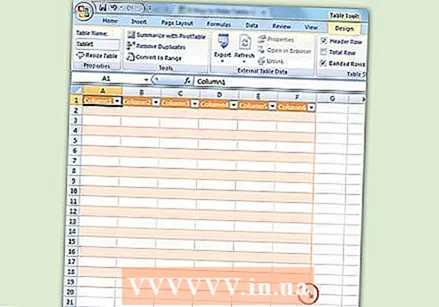1. Grab the corner of the table. Move the mouse cursor over the resize handle in the lower right corner of the table. The cursor will change to a 2-sided diagonal arrow. Press and hold this button to grab the corner.
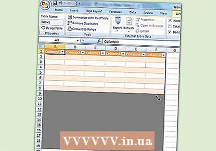2. Change the size of the table. Drag the cursor in to shrink the table, out to enlarge it. Dragging changes the number of rows and columns.
   • Dragging the cursor up towards the column header decreases the number of rows in the table, while dragging the cursor down increases the number of rows.
   • Dragging the cursor to the left decreases the number of columns in the table, while dragging to the right increases the number of columns. A new header is created when a new column is added.

Part 3 of 8: Inserting and removing table rows and columns

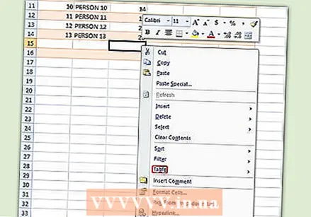
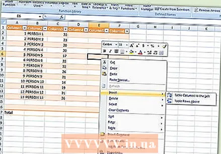
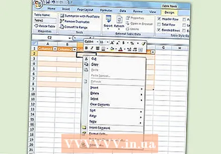1. Right-click on the table cell where you want to insert or delete a row or column. A pop-up menu will appear.
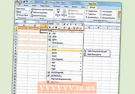2. Select "Insert" from the pop-up menu. Choose one of the options from the Insert submenu.
   • Select "Insert Columns to the Left" or "Insert Columns to the Right" to add a new column to the table.
   • Select "Insert Rows Above" or "Insert Rows Below" to add a new row to the table.
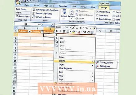3. Select "Delete" from the pop-up menu. Choose one of the options from the Delete submenu.
   • Select "Table Columns" to delete entire columns of the selected cells.
   • Select "Table Rows" to delete entire rows with the selected cells.

Part 4 of 8: Sorting table rows

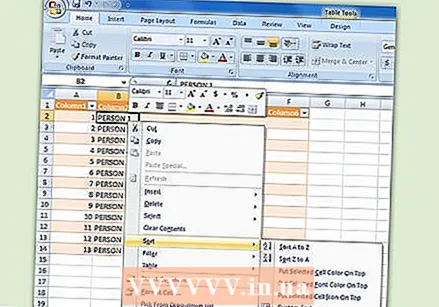
1. Click the down arrow to the right of the heading of the column you want to sort. A drop-down menu will appear.
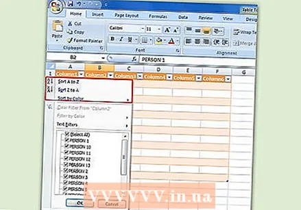2. Choose one of the sort options displayed. The sort options appear at the top of the drop-down menu.
   • Choose "Sort A to Z" (or "Sort Smallest to Largest" if the data is numeric) to sort items in ascending order.
   • Choose "Sort Z to A" (or "Sort Largest to Smallest" if the data is numeric) to sort items in descending order.
   • Choose "Sort By Color" and then select "Custom Sort" from the submenu to start a custom sort. If your data is shown in multiple colors, you can choose a color to sort the data by.
3. Access to additional options. You can find additional sort options by right-clicking on any cell in a column and choosing "Sort" from the pop-up menu. In addition to the above options, you can also sort by cell or letter color.

Part 5 of 8: Filtering data in tables

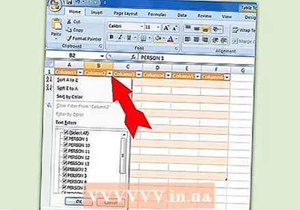
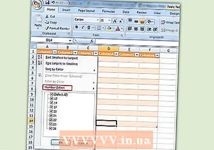1. Click the down arrow to the right of the header of the column you want to filter. A drop-down menu will appear.
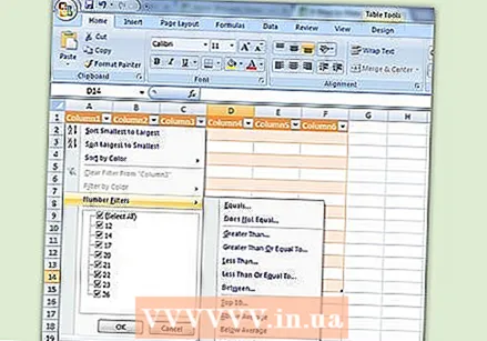2. Choose one of the filter options that are displayed. Three filter options are available: "Filter by Color," "Text Filters," and "Number Filters." (The "Text Filters" option is only shown when the columns contain text, while the "Number Filters" option is only shown when the columns contain numbers.) Below that you will find a series of checkboxes.
   • The option "Filter by Color" is active when the text or numbers are displayed in multiple colors. Select the color for which you want to filter out the data.
   • The "Text Filters" option also includes "Equals," "Does Not Equal," "Greater Than," "Begins With," "Ends With," "Contains," "Does Not Contain", and "Custom Filter" options.
   • The "Number Filters" option also includes the options "Equals", "Does Not Equal," "Greater Than," "Greater Than or Equal To," "Less Than," "Less Than of Equal To," "Between," "Top 10," "Above Average," "Below Average" and "Custom Filter".
   • The checkboxes below these options consist of "Select All" and the option "Blanks" to show all data that matches the filters or all rows with empty cells, in addition to a list of every unique data element (such as the same name) in that column. . Check the combination of boxes to show only those rows with cells that meet the set criteria, such as checking elements like "Smith" and "Jones" to show the numbers of only those two people.
   • Excel 2010 and 2013 offer an additional filter option: enter text or a number in the search field and only those rows will be shown with an item in the column that matches the value in the search field.
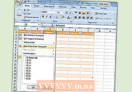3. Remove the filter when you are done with it. To restore the original overview, select "Clear Filter From [Column Name]" from the drop-down menu. (The actual name of the column is shown by this option.)

Part 6 of 8: Adding a Totals row to a table

1. Right-click on any cell in the table. This will display a context menu. Select "Table" from the pop-up menu.
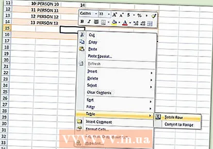2. Select "Totals Row" from the Table submenu. A Totals row appears below the last row of the table, a total of all numeric data in each column.
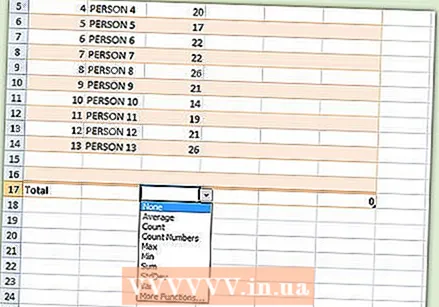3. Change the displayed value. Click the menu on the totals line for the value you want to adjust. You can choose which function you want to display. You can display the sum, the average and the total, among other things.

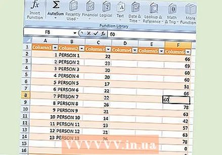
Part 7 of 8: Add a calculation column to a table

1. Select a cell in an empty column. If necessary, you must first add an empty column. For the methods to do this, see "Expanding and Shrinking the Table" and "Inserting and Deleting Table Rows and Columns".
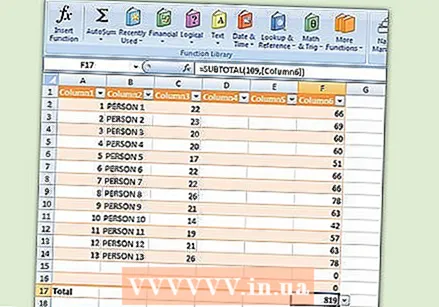2. Enter the formula for the calculation in the blank cell, but not in the header. Your formula is automatically copied to all cells of the column, both above and below the cell where you entered the formula. You can also do this manually.
   • You can enter the formula in any row of the worksheet below the table, but you cannot reference cells in those rows in the table reference.
   • You can type in the formula or move it to a column that already contains data, but to turn it into a calculation column, you must click the "AutoCorrect Options" option to overwrite existing data. If you copy the formula, you will have to manually overwrite data by copying the formula to those cells.
3. Make exceptions. After creating a calculation column, you can go back and make exceptions at a later stage by typing data other than a formula into cells, which will delete the formula in those cells, or you can copy another formula to cells. Exceptions to the calculation column formula other than a formula deletion are clearly marked.

Part 8 of 8: Changing the style of the table

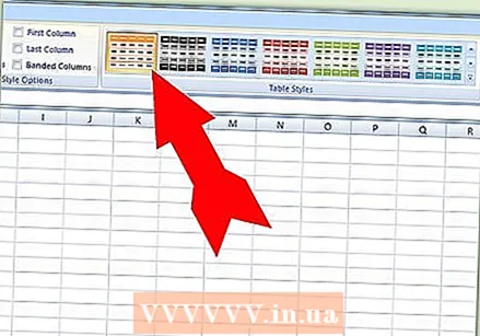1. Select a predefined style. You can choose from a number of preset color combinations for your table. Click anywhere in the table to select it, then click the Design tab if it is not already open.
   • Choose from one of the available styles in Table Styles. Click the More button on the right and expand the list to see all options.
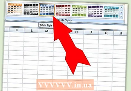2. Create a custom style. Click the More button on the right side of the list of preset styles. Click on “New Table Style” at the bottom of the menu. This will open the “New Table Quick Style” window.
   • Name your style. If you want to find the new style quickly, give it a name that you can remember or that describes the style well.
   • Choose the element you want to adjust. You will see a list of table elements. Choose the element you want to edit and click the “Format” button.
   • Choose the properties for the layout of the element. You can adjust the font, fill color and style of the borders. This formatting will be applied to the element you selected.
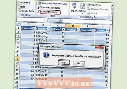3. Change your table back to a normal worksheet. When you have finished working with the data in a separate table, you can convert it back to a normal worksheet, without losing any data. Click anywhere in the table to select it.
   • Click the Design tab.
   • Click Convert to Range and then Yes.
   • The table formatting will be removed, but the style will remain. It is no longer possible to sort and / or filter data.

Tips

• If you no longer need the table, you can delete it completely or turn it back into a series of data in your worksheet. To completely delete the table, select the table and press the "Delete" key. To turn it back into a range of data, right-click on one of the cells, select "Table" from the pop-up menu, then select "Convert to Range" from the Table submenu. The sort and filter arrows disappear from the column headers, and the table references in the cell formulas are removed. The column headings and the formatting of the table are preserved.
• If you place the table so that the column header is in the top left corner of the worksheet (cell A1), the column headers will replace the worksheet headers when you scroll up. If you move the table elsewhere, the column headers will scroll out of sight when you scroll up, and you will have to use Freeze Panes to display them continuously

.