Content

• To step
• Method 1 of 3: Using Conditional Formatting in Windows
• Method 2 of 3: Using conditional formatting on a Mac
• Method 3 of 3: Using a table style

This wikiHow teaches you how to select alternate rows in Microsoft Excel for Windows or macOS.

To step

Method 1 of 3: Using Conditional Formatting in Windows

1. Open the spreadsheet you want to edit in Excel. You can usually do this by double-clicking the file on your PC.
   • This method is suitable for all types of data. You can adjust your data as needed without affecting the layout.
2. Select the cells you want to format. Click and drag the mouse so that all cells in the range you want to format are selected.
   • To select every other row in the whole document, click the button Select all, the gray square button / cell in the top left corner of the sheet.
3. Click on it click on New rule. This will open the "New Formatting Rule" dialog box.
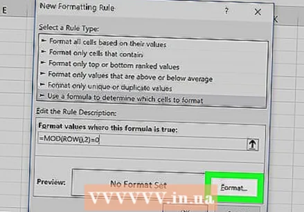
4. Select Use a formula to determine which cells are formatted. This option is under "Select a rule type."
   • in Excel 2003, you set "condition 1" as "Formula is".
5. Enter the formula to select alternate rows. Enter the following formula in the field:
   • = MOD (ROW (), 2) = 0
6. click on Formatting. This is a button at the bottom of the dialog.
7. Click on the tab Padding. You can find this at the top of the dialog box.
8. Select a pattern or color for the selected rows and click OK. You can see an example of the color below the formula.
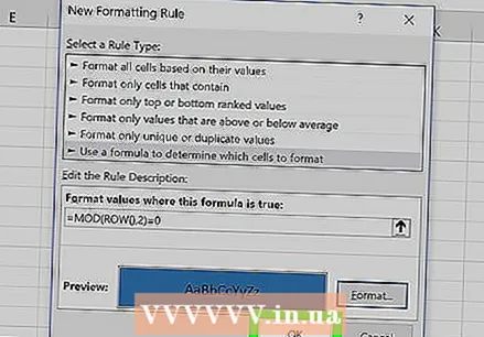9. click on OK. This highlights alternating rows in the spreadsheet with the color or pattern you selected.
   • You can edit your formula or format by clicking the arrow next to Conditional Formatting (in the Home tab), Manage rules and then select the line.

Method 2 of 3: Using conditional formatting on a Mac

1. Open the spreadsheet you want to edit in Excel. You can usually do this by double-clicking the file on your Mac.
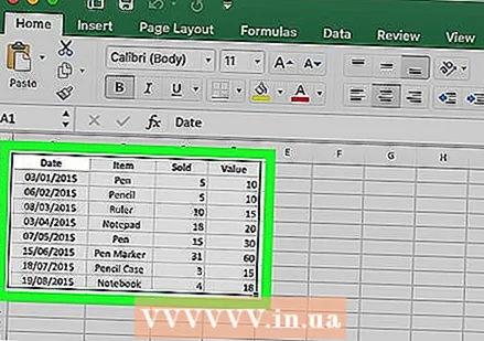2. Select the cells you want to format. Click and drag the mouse to select all cells in the range that you want to edit.
   • To select every other row in the whole document, press ⌘ Command+a on your keyboard. This will select all cells in your spreadsheet.
3. Click on it 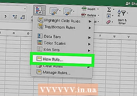click on New rule from the menu "Conditional Formatting. This will open your formatting options in a new dialog titled "New Formatting Rule".
4. Select Classic next to Style. Click the drop-down list of Style in the pop-up window, and select Classic at the bottom of the menu.
5. Select Use a formula to determine which cells are formatted under Style. Click the drop-down under the Style option, and select the option Using a Formula to customize the formatting with a formula.
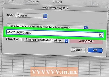6. Enter the formula to select alternate rows. Click the formula field in the New Formatting Rule window and type the following formula:
   • = MOD (ROW (), 2) = 0
7. Click the drop-down list next to Format with. You can find this option under the formula field at the bottom. You will now see more formatting options in a list.
   • The formatting you select here will be applied to every other row in the selected area.
8. Select a formatting option from the "Format With" menu. You can click on an option here and view it on the right side of the pop-up window.
   • If you want to manually create a new selection layout with a different color, click the option Custom layout at the bottom of. A new window will open and you can manually select fonts, borders and colors to use.
9. click on OK. Your custom formatting is applied and every other row in the selected area of ​​your spreadsheet is now selected.
   • You can edit the rule at any time by clicking the arrow next to Conditional Formatting (in the Home tab), Manage rules and then select the line.

Method 3 of 3: Using a table style

1. Open the spreadsheet you want to edit in Excel. You can usually do this by double-clicking the file on your PC or Mac.
   • Use this method if you want to add your data to a browsable table in addition to selecting every other row.
   • Only use this method if you don't need to edit the data in the table after applying the style.
2. Select the cells you want to add to the table. Click and drag the mouse so that all cells in the range that you want to style are selected.
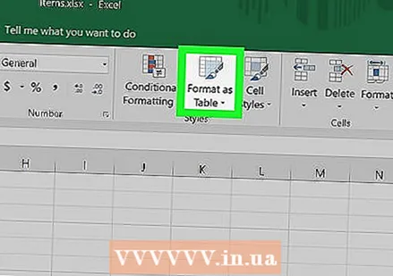3. click on Format as table. This is in the Home tab on the toolbar at the top of Excel.
4. Select a table style. Scroll through the options in the Light, Medium, and Dark groups, then click the one you want to use.
5. click on OK. This applies the style to the selected data.
   • You can edit the style of the table by selecting or deselecting preferences in the "Table Style Options" panel on the toolbar. If you don't see this panel, click a cell in the table to make it appear.
   • If you want to convert the table back to a normal range of cells so that you can edit the data, click the table to bring up the table tools in the toolbar, click the tab Design then click Convert to range.