Content

• To step
• Part 1 of 2: Create a line chart
• Part 2 of 2: Editing your chart
• Tips
• Warnings

In this article, you can read how to create a line chart with data in Excel. This can be done on a PC with Windows as well as on a Mac.

To step

Part 1 of 2: Create a line chart

1. Open Excel. Click twice on the Excel icon. It looks like a white letter "X" on a green folder. This will open the Excel home page.
   • If you already have an Excel file with data, click on the file and skip the two steps below.
2. click on Blank worksheet. You can find this option on the home page of Excel. This is how you open a new worksheet in Excel for your data.
   • On a Mac, depending on your settings, you may automatically see a blank worksheet. If so, skip this step.
3. Enter your details. A line chart must consist of two axes. Enter your details in two columns. For convenience, put the data for the X-axis (time) in the left column and the data you've collected in the right column.
   • For example, if you want to see how much you have spent during a year, put that date in the left column and your expenses in the right column.
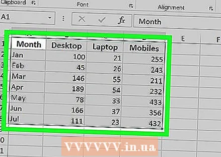4. Select your data. Click on the top left cell and drag your mouse to the bottom right cell in the group of data. This is how you select all your data.
   • Don't forget to select the column headings as well, if applicable.
5. Click on the tab Insert. You can find it to the left of the green ribbon at the top of the Excel window. This will open the taskbar Insert under the green ribbon.
6. Click on the "Line chart" icon. It is the box with multiple lines drawn on it in group of options for Diagrams. A drop-down menu will then appear.
7. Choose a style for your diagram. Swipe your mouse cursor over any of the sample graphs you see in the drop-down menu to see what a particular menu would look like with your data. You should see a small window with a graph on it appear in the middle of your Excel window.
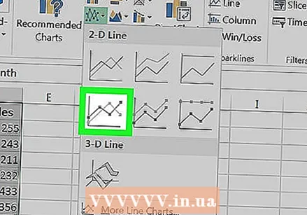8. Click on a type of diagram. Once you have chosen a model, click on it to create your line chart. It will be placed in the middle of the Excel window.

Part 2 of 2: Editing your chart

1. Edit the design of your chart. Once you have created your chart, a toolbar with the title will appear Design. You can edit the design and appearance of your chart by clicking one of the variations in the "Chart Styles" section on the toolbar.
   • If this taskbar does not open, click on your chart and then click on the tab To design in the green ribbon.
2. Move your line chart. Click on the white space almost at the top of the line chart and drag the chart to where you want it.
   • You can also move specific parts of the line chart (for example, the title) by clicking and dragging them around within the line chart window.
3. Make the graph bigger or smaller. Click on one of the circles on one of the corners of the graph window and drag it in or out to make the graph larger or smaller.
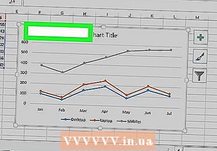
4. Adjust the title of the chart. Click twice on the title of the chart, then select the text "Chart name" and type in the title of your chart. Save the text by clicking anywhere outside the chart name field.
   • You can also do this with the titles of the graph axes.

Tips

• You can add data to your chart in a new column, then select and copy it and paste it into the chart window.

Warnings

• Some charts are specially designed for specific types of data (such as percentages, or money). Make sure that the model you have chosen does not already contain a topic before you start making your graph.