Content

• Steps
• Tips
• Warnings

Microsoft Excel provides functions for calculating various financial transactions, including payments of principal and interest on loans and investments. Due to the fact that some loans only require interest payments, knowing how to calculate interest payments is critical to budgeting. You can also have a deposit that pays monthly or quarterly interest - in this case, the calculation of such a payment can be performed in the same way to determine how much income will be received. Calculating all kinds of interest payments in Excel is easy. See step 1 below to get started.

Steps

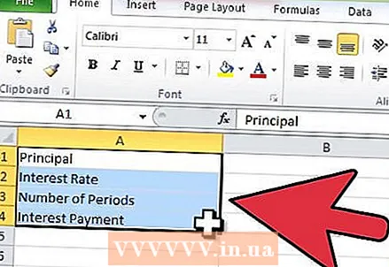1. 1 Set up your spreadsheet for calculating interest payments.
   • Create labels in cells A1: A4 as follows: Principal, Interest Rate, Number of Periods, and Interest Payment.
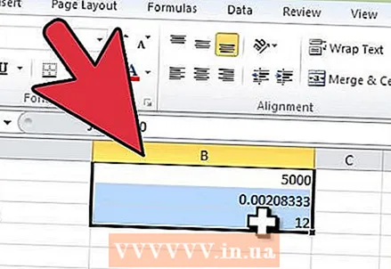2. 2 Enter your transaction information in cells B1 down to B3.
   • Enter the principal or deposit amount in cell "Principal," B1.
   • Divide your annual interest rate by 12 if you want to calculate interest on a monthly basis; divide by 4 if the quarterly percentage is to be calculated. Place it in cell B2.
   • The number of periods involved in your loan or deposit goes to cell B3. If the calculation of interest payments for a deposit with an indefinite duration - use the number of interest payments per year. This will be the same number divided by the interest rate in the Interest Rate box.
   • For example, suppose you are calculating a monthly interest payment of $ 5,000 at 2.5 percent per annum. Enter "5000" "in cell B1," = .025 / 12 "" in cell B2 and "1" "in cell B3.
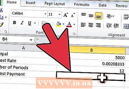3. 3 Select cell B4 by clicking on it.
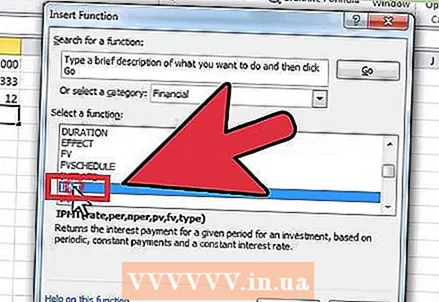4. 4 Insert the IPMT function for calculating interest payments.
   • Click the function shortcut button on the toolbar labeled "fx."
   • Enter "interest payment" in the text input field and click "Go."
   • Select the "IPMT" function from the list below and then click the "OK." The "Function Argument" window will open.
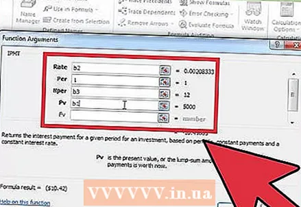5. 5 Refer to the appropriate cells for each part of the parameter.
   • In the field "Rate" enter "B2," "B3" is entered in the field "Nper" and "B1" is entered in the field "PV".
   • The value in the "Per" field must be "1."
   • Leave the "FV" field blank.
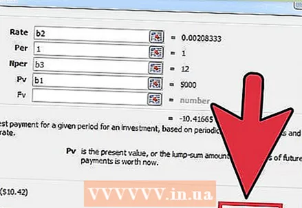6. 6 Click the "OK" button to complete the process of entering information in the "Function Arguments" window and to show the interest payment amount.
   • Note that this value is negative as it refers to the money that is being paid.
7. 7 Ready.

Tips

• You can copy and paste cells A1: B4 to another part of the table in order to evaluate the changes made by different interest rates and terms without losing the original formula and result.

Warnings

• Make sure you enter the interest rate as a decimal and you divide it by the number of times by which the transaction interest is calculated during the calendar year.