Content

• To step
• Method 1 of 3: Understanding VLOOKUP
• Method 2 of 3: Understand the VLOOKUP values
• Method 3 of 3: Using VLOOKUP
• Tips

It seems like using the VLOOKUP function in Microsoft Excel is only for professionals, but it's actually really easy to do. Just by learning a little bit of code, you can make getting information from any spreadsheet much easier.

To step

Method 1 of 3: Understanding VLOOKUP

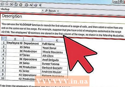1. Know when to use VLOOKUP. VLOOKUP is a function in Excel that allows you to type in the value of a cell to find the value of a corresponding cell in the same row.
   • Use this if you are looking for data in a large spreadsheet or if you are looking for repetitive data.
   • Imagine you are a teacher with a student list in Excel. You can use VLOOKUP to type in a student's name and instantly get their grade from a corresponding cell.
   • VLOOKUP is useful if you work in retail. You can search for an item by its name and you will get the item number or price as a result.
2. Make sure your spreadsheet is properly organized. The "v" in VLOOKUP stands for "vertical." This means that your spreadsheet must be organized in vertical lists, as the function only searches columns, not rows.
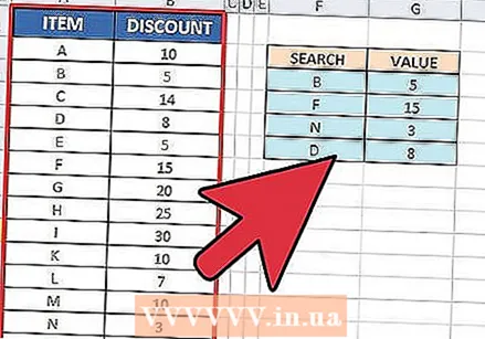3. Use VLOOKUP to find a discount. If you're using VLOOKUP for the business, you can format it into a table that calculates the price or discount on a particular item.

Method 2 of 3: Understand the VLOOKUP values

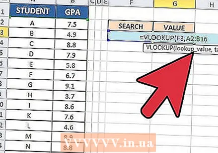
1. Understand the “search value.This is the cell from which you begin; where you enter the code for VLOOKUP.
   • This is the number of a cell, such as F3. This refers to the search location.
   • You enter the code of VLOOKUP here. Whatever search value you enter here must come from the first column of your spreadsheet.
   • It's helpful to remove this a few cells from the rest of the worksheet so that you don't confuse it with the rest of the data.
2. Understand what the “table matrix” is. These are the cells of the entire data range.
   • The first number is the top left corner of the worksheet and the second number is the bottom right corner of your data.
   • We take again the example of the teacher and the student list. Suppose you have 2 columns. In the first are the names of the students and in the second their average grade. If you have 30 students, starting in A2, the first column of A2-A31 will run. The second column with the numbers goes from B2-B31. So the table array is A2: B31.
   • Make sure you do not include the column headings. This means that you do not include the name of each column in your table matrix, such as “Student Name” and “Avg. figure". These will likely be A1 and B1 in your worksheet.
3. Find the “column index.This is the number of the column where you are looking for the data.
   • For VLOOKUP to work you will have to use the column number and not the name. So even if you search through the students' average grades, you still put a “2” as the column index number, because the average grade is in that column.
   • Do not use the letter for this, only the number that belongs to the column. VLOOKUP will not recognize a "B" as the correct column, only a "2."
   • You may have to literally count which column to use as the column index if you are working with a very large spreadsheet.
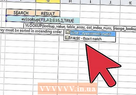4. Understand what "approach" means. This is the part of VLOOKUP where you can indicate whether you are looking for an exact number or an estimated number.
   • If you want an exact number and not a number that has been rounded, you must indicate “FALSE” in the VLOOKUP function.
   • If you want an estimated value that has been rounded off or borrowed from a neighboring cell, put “TRUE” in the function.
   • If you are not sure what you need, it is usually safe to use “FALSE” to get an exact answer to your worksheet search.

Method 3 of 3: Using VLOOKUP

1. Create the worksheet. You need at least 2 columns of data for the VLOOKUP function to work, but you can use as many as you want
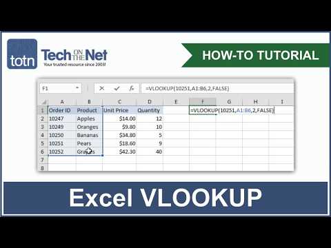
2. In an empty cell, type the VLOOKUP formula. In the cell, enter the following formula: = VLOOKUP (lookupvalue, table_array, column_index_num, [approximate]).
   • You can use any cell you want for this, but be sure to use that cell's value as the “lookup value” in your function code.
   • See the guide above for information on what each of the values ​​in the function should do. We follow the example of the Student List again with the values ​​discussed earlier, which makes the VLOOKUP formula look like this: = VLOOKUP (F3, A2: B32,2, FALSE)
3. Expand VLOOKUP to include more cells. Select the cell within the VLOOKUP code. In the bottom right corner, select the handle of the cell and drag it to include one or more extra cells in the matrix.
   • This allows you to search with VLOOKUP, because you need at least 2 columns for data input / output.
   • You can place the target of any cell in an adjacent (but not shared) cell. For example, on the left side of the course in which you are looking for a student, you can put “Student name”.
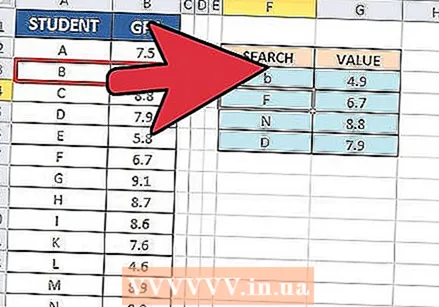4. Test VLOOKUP. You do this by entering the search value. In the example, this is the student's name, entered in one of the cells as included in the VLOOKUP code. After that, VLOOKUP should automatically return the said student's average grade in the adjacent cell.

Tips

• To prevent the VLOOKUP code from changing the value of the cell when you edit or add cells in the table, put a "$" in front of each letter / number of your table array. For example, our VLOOKUP code changes to = VLOOKUP (F3, $ A $ 2: $ B $ 32.2, FALSE)
• Do not include spaces before or after the data in the cells, or incomplete, inconsistent quotation marks.