Content

• To step
• Method 1 of 2: Hide a selection of rows
• Method 2 of 2: Hide grouped rows

Hiding rows and columns you don't need can make your Excel spreadsheet much easier to read, especially if it's a large file. Hidden rows don't clutter your worksheet, but are still included in formulas. You can easily hide and unhide rows in any version of Excel by following this guide.

To step

Method 1 of 2: Hide a selection of rows

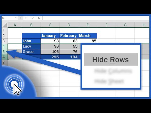
1. Use the row selection tool to highlight the rows you want to hide. You can hold down the Ctrl key to select multiple rows.
2. Right click inside the highlighted area. Select "Hide". The rows in the worksheet are hidden.
3. Make the rows visible again. To unhide the rows, first select the rows to highlight the rows above and below the hidden rows. For example, select row four and row eight if rows 5-7 are hidden.
   • Right click inside the highlighted area.
   • Select "Unhide".

Method 2 of 2: Hide grouped rows

1. Create a group of rows. Excel 2013 allows you to group / ungroup rows so that you can easily hide and unhide them.
   • Highlight the rows you want to group and click the "Data" tab.
   • Click the "Group" button in the "Overview" group.
2. Hide the group. A line and a box with a minus sign (-) appear next to those rows. Click the box to hide the "grouped" rows. Once the rows are hidden, the small box will show a plus sign (+).
3. Make the rows visible again. Click on the plus (+) if you want to make the rows visible again.