Content

• To step
• Part 1 of 4: Drawing up the matrix
• Part 2 of 4: Learning the operations for solving a system with a matrix
• Part 3 of 4: Merge the steps to solve the galaxy
• Part 4 of 4: Checking your solution
• Tips

A matrix is ​​a very useful way of representing numbers in a block format, which you can then use to solve a system of linear equations. If you only have two variables, you will likely use a different method. Read about this in Solving a System of Equations for examples of these other methods. But if you have three or more variables, an array is ideal. By using repeated combinations of multiplication and addition, you can systematically arrive at a solution.

To step

Part 1 of 4: Drawing up the matrix

1. Verify that you have sufficient data. To get a unique solution for every variable in a linear system using a matrix, you need to have as many equations as the number of variables you are trying to solve. For example: with the variables x, y and z you need three equations. If you have four variables, you need four equations.
   • If you have fewer equations than the number of variables, you will find some boundaries of the variables (such as x = 3y and y = 2z), but you cannot get a precise solution. For this article we will only work towards a unique solution.
2. Write your equations in the standard form. Before you can put data from the equations in a matrix form, you first write each equation in standard form. The standard form for a linear equation is Ax + By + Cz = D, where the uppercase letters are the coefficients (numbers), and the last number (the D in this example) is to the right of the equal sign.
   • If you have more variables, just continue the line for as long as you need to. For example, if you were trying to solve a system with six variables, your default shape would look like Au + Bv + Cw + Dx + Ey + Fz = G. In this article we will focus on systems with only three variables. Solving a larger galaxy is exactly the same, but just takes more time and more steps.
   • Note that in standard form, the operations between the terms is always an addition. If there is a subtraction in your equation, instead of an addition, you will have to work with this later by making your coefficient negative. To make this easier to remember, you can rewrite the equation and add the operation and make the coefficient negative. For example, you can rewrite the equation 3x-2y + 4z = 1 as 3x + (- 2y) + 4z = 1.
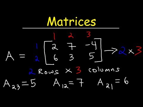
3. Place the numbers from the system of equations in a matrix. A matrix is ​​a group of numbers, arranged in a kind of table, with which we will work to solve the system. It basically contains the same data as the equations themselves, but in a simpler format. To make the matrix of your equations in standard form, just copy the coefficients and result of each equation into a single row, and stack those rows on top of each other.
   • Suppose you have a system consisting of the three equations 3x + y-z = 9, 2x-2y + z = -3, and x + y + z = 7. The top row of your matrix will contain the numbers 3, 1, -1, 9, as these are the coefficients and the solution of the first equation. Note that any variable that does not have a coefficient is assumed to have a coefficient of 1. The second row of the matrix becomes 2, -2, 1, -3 and the third row becomes 1, 1, 1, 7.
   • Make sure to align the x coefficients in the first column, the y coefficients in the second, the z coefficients in the third, and the solution terms in the fourth. When you are done working with the matrix, these columns will be important when writing your solution.
4. Draw a large square bracket around your entire matrix. By convention, a matrix is ​​indicated by a pair of square brackets, [], around the entire block of numbers. The brackets do not affect the solution in any way, but they do indicate that you are working with matrices. A matrix can consist of any number of rows and columns. In this article, we will use parentheses around terms in a row to indicate that they belong together.
5. Use of common symbolism. When working with matrices, it is common to refer to the rows with the abbreviation R and the columns with the abbreviation C. You can use numbers along with these letters to indicate a specific row or column. For example, to indicate row 1 of a matrix, you can write R1. Row 2 then becomes R2.
   • You can indicate any specific position in a matrix using a combination of R and C. For example, to indicate a term in the second row, third column, you could call it R2C3.

Part 2 of 4: Learning the operations for solving a system with a matrix

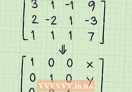1. Understand the shape of the solution matrix. Before you start solving your system of equations, you need to understand what you are going to do with the matrix. At this point you have a matrix that looks like this:
   • 3 1 -1 9
   • 2 -2 1 -3
   • 1 1 1 7
   • You work with a number of basic operations to create the "solution matrix". The solution matrix will look like this:
   • 1 0 0 x
   • 0 1 0 y
   • 0 0 1 z
   • Note that the matrix consists of 1's in a diagonal line with 0's in all other spaces except the fourth column. The numbers in the fourth column are the solution for the variables x, y and z.
2. Use scalar multiplication. The first tool at your disposal to solve a system using a matrix is ​​scalar multiplication. This is simply a term that means that you multiply the elements in a row of the matrix by a constant number (not a variable). When using scalar multiplication, keep in mind that you must multiply each term of the entire row by whatever number you select. If you forget the first term and just multiply, you will get the wrong solution. However, you don't have to multiply the entire matrix at the same time. In scalar multiplication, you only work on one row at a time.
   • It is common to use fractions in scalar multiplication because you often want to get a diagonal row of 1's. Get used to working with fractions. It will also be easier (for most of the steps in solving the matrix) to be able to write your fractions in improper form, then convert them back to mixed numbers for the final solution. Therefore, the number 1 2/3 is easier to work with if you write it as 5/3.
   • For example, the first row (R1) of our example problem starts with the terms [3,1, -1,9]. The solution matrix must contain a 1 in the first position of the first row. To "change" the 3 to a 1, we can multiply the entire row by 1/3. This creates the new R1 of [1,1 / 3, -1 / 3,3].
   • Make sure to leave any negative signs where they belong.
3. Use row addition or row subtraction. The second tool you can use is to add or subtract two rows of the matrix. To create the 0 terms in your solution matrix, you have to add or subtract numbers to get to the 0. For example, if R1 is of a matrix [1,4,3,2] and R2 is [1,3,5,8], then you can subtract the first row from the second row and create a new row [0, -1, 2.6], because 1-1 = 0 (first column), 3-4 = -1 (second column), 5-3 = 2 (third column), and 8-2 = 6 (fourth column). When performing a row addition or row subtraction, rewrite your new result instead of the row you started with. In this case we would extract row 2 and insert the new row [0, -1,2,6].
   • You can use a shorthand notation and declare this action as R2-R1 = [0, -1,2,6].
   • Remember that addition and subtraction are just opposite forms of the same operation. Think of it as adding two numbers or subtracting the opposite. For example, if you start with the simple equation 3-3 = 0, you can think of this as an addition problem of 3 + (- 3) = 0. The result is the same. This seems simple, but it is sometimes easier to consider a problem in one form or another. Just keep an eye on your negative signs.
4. Combine row addition and scalar multiplication in a single step. You cannot expect the terms to always match, so you can use a simple addition or subtraction to create 0's in your matrix. More often you will have to add (or subtract) a multiple from another row. To do this, you first do the scalar multiplication, then add that result to the target row you are trying to change.
   • Suppose; that there is a row 1 of [1,1,2,6] and a row 2 of [2,3,1,1]. You want a 0 term in the first column of R2. That is, you want to change the 2 to a 0. To do this, you must subtract a 2. You can get a 2 by first multiplying row 1 by the scalar multiplication 2, and then subtracting the first row from the second row. In short form this can be written down as R2-2 * R1. First, multiply R1 by 2 to get [2,2,4,12]. Then subtract this from R2 to get [(2-2), (3-2), (1-4), (1-12)]. Simplify this and your new R2 will be [0,1, -3, -11].
5. Copy rows that remain unchanged as you work. As you work on the matrix, you will change a single row at a time, either by scalar multiplication, row addition, or row subtraction, or a combination of steps. When you change one row, make sure to copy the other rows of your matrix in their original form.
   • A common error occurs when performing a combined multiplication and addition step in one move. For example, say you need to subtract R1 from R2 twice. When you multiply R1 by 2 to do this step, remember that R1 does not change in the matrix. You only do the multiplication to change R2. First copy R1 in its original form, then make the change to R2.
6. First work from top to bottom. To solve the system, you work in a very organized pattern, essentially "solving" one term of the matrix at a time. The sequence for a three-variable array will look like this:
   • 1. Make a 1 in the first row, first column (R1C1).
   • 2. Make a 0 in the second row, first column (R2C1).
   • 3. Make a 1 in the second row, second column (R2C2).
   • 4. Make a 0 in the third row, first column (R3C1).
   • 5. Make a 0 in the third row, second column (R3C2).
   • 6. Make a 1 in the third row, third column (R3C3).
7. Work back from the bottom to the top. At this point, if you did the steps correctly, you are halfway through the solution. You must have the diagonal line of 1's, with 0's below it. The numbers in the fourth column don't matter at this point. Now you work as follows back to the top:
   • Create a 0 in the second row, third column (R2C3).
   • Create a 0 in the first row, third column (R1C3).
   • Create a 0 in the first row, second column (R1C2).
8. Check if you have created the solution matrix. If your work is correct, you have created the solution matrix with 1's in a diagonal line of R1C1, R2C2, R3C3 and 0's in the other positions of the first three columns. The numbers in the fourth column are the solutions for your linear system.

Part 3 of 4: Merge the steps to solve the galaxy

1. Start with an example system of linear equations. To practice these steps, let's start with the system we used earlier: 3x + y-z = 9, 2x-2y + z = -3, and x + y + z = 7. If you write this in a matrix, you have R1 = [3,1, -1,9], R2 = [2, -2,1, -3], and R3 = [1,1,1,7].
2. Create a 1 in the first position R1C1. Note that R1 starts with a 3 at this point. You have to change it to a 1. You can do this by scalar multiplication, multiplying all four terms of R1 by 1/3. In shorthand you can write as R1 * 1/3. This gives a new result for R1 if R1 = [1,1 / 3, -1 / 3,3]. Copy R2 and R2, unchanged, when R2 = [2, -2,1, -3] and R3 = [1,1,1,7].
   • Note that multiplication and division are only inverse functions of each other. We can say that we multiply by 1/3 or divide by 3, without changing the result.
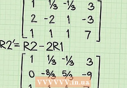3. Create a 0 in the second row, first column (R2C1). At this point, R2 = [2, -2,1, -3]. To get closer to the solution matrix, you need to change the first term from a 2 to a 0. You can do this by subtracting twice the value of R1, since R1 starts with a 1. In shorthand, the operation R2- 2 * R1. Remember, you don't change R1, just work with it. So first copy R1 if R1 = [1,1 / 3, -1 / 3,3]. Then if you double each term of R1, you get 2 * R1 = [2,2 / 3, -2 / 3,6]. Finally, subtract this result from the original R2 to get your new R2. Working term by term, this subtraction becomes (2-2), (-2-2 / 3), (1 - (- 2/3)), (-3-6). We simplify these to the new R2 = [0, -8 / 3,5 / 3, -9]. Note that the first term is 0 (whatever your goal was).
   • Write row 3 (which has not changed) as R3 = [1,1,1,7].
   • Be careful when subtracting negative numbers to make sure the signs stay correct.
   • Now first let's leave the fractions in their improper form. This makes later steps of the solution easier. You can simplify the fractions in the last step of the problem.
4. Create a 1 in the second row, second column (R2C2). To keep forming the diagonal line of 1's, you must convert the second term -8/3 into 1. Do this by multiplying the entire row by the reciprocal of that number (-3/8). Symbolically, this step is R2 * (- 3/8). The resulting second row is R2 = [0.1, -5 / 8.27 / 8].
   • Note that if the left half of the row starts to resemble the solution with the 0 and 1, the right half may start to look ugly, with improper fractions. For now, just leave them for what they are.
   • Don't forget to continue copying the untouched rows, so R1 = [1,1 / 3, -1 / 3,3] and R3 = [1,1,1,7].
5. Create a 0 in the third row, first column (R3C1). Your focus now moves to the third row, R3 = [1,1,1,7]. To make a 0 in the first position, you must subtract a 1 from the 1 currently in that position. If you look up, there is a 1 on the first position of R1. So you just need to subtract R1 from R3 to get the result you need. Working term for term, this becomes (1-1), (1-1 / 3), (1 - (- 1/3)), (7-3). These four mini-problems can then be simplified to the new R3 = [0.2 / 3.4 / 3.4].
   • Continue to copy along R1 = [1.1 / 3, -1 / 3.3] and R2 = [0.1, -5 / 8.27 / 8]. Remember you only change one row at a time.
6. Make a 0 in the third row, second column (R3C2). This value is currently 2/3, but must be converted to a 0. At first glance, it looks like you can subtract the R1 values ​​by double, since the corresponding column of R1 contains a 1/3. However, if you double and subtract all the values ​​of R1, the 0 in the first column of R3 changes, which you don't want. This would be a step back in your solution. So you have to work with some combination of R2. Subtracting 2/3 from R2 creates a 0 in the second column without changing the first column. In short form this is R3-2 / 3 * R2. The individual terms become (0-0), (2 / 3-2 / 3), (4/3 - (- 5/3 * 2/3)), (4-27 / 8 * 2/3) . Simplification then gives R3 = [0,0,42 / 24,42 / 24].
7. Create a 1 in the third row, third column (R3C3). This is a simple multiplication by the reciprocal of the number that it says. The current value is 42/24, so you can multiply by 24/42 to get the value you want 1. Note that the first two terms are both 0, so any multiplication remains 0. The new value of R3 = [0,0,1,1].
   • Note that the fractions that seemed quite complicated in the previous step are already starting to resolve.
   • Continue with R1 = [1.1 / 3, -1 / 3.3] and R2 = [0.1, -5 / 8.27 / 8].
   • Note that at this point you have the diagonal of 1's for your solution matrix. You only have to convert three elements of the matrix into 0s to find your solution.
8. Create a 0 in the second row, third column. R2 is currently [0.1, -5 / 8.27 / 8], with a value of -5/8 in the third column. You have to transform it to a 0. This means that you have to perform some operation with R3 that consists of adding 5/8. Since the corresponding third column of R3 is a 1, you must multiply all the values ​​of R3 by 5/8 and add the result to R2. In short, this is R2 + 5/8 * R3. Term for term this is R2 = (0 + 0), (1 + 0), (-5 / 8 + 5/8), (27/8 + 5/8). This can be simplified to R2 = [0,1,0,4].
   • Then copy R1 = [1,1 / 3, -1 / 3,3] and R3 = [0,0,1,1].
9. Create a 0 in the first row, third column (R1C3). The first row is currently R1 = [1,1 / 3, -1 / 3,3]. You have to convert the -1/3 in the third column to a 0, using some combination of R3. You don't want to use R2, because the 1 in the second column of R2 would change R1 the wrong way. So you multiply R3 * 1/3 and add the result to R1. The notation for this is R1 + 1/3 * R3. The term for term elaboration results in R1 = (1 + 0), (1/3 + 0), (-1 / 3 + 1/3), (3 + 1/3). You can simplify this to a new R1 = [1,1 / 3,0,10 / 3].
   • Copy the unchanged R2 = [0,1,0,4] and R3 = [0,0,1,1].
10. Make a 0 in the first row, second column (R1C2). If everything is done correctly, this should be the last step. You have to convert 1/3 in the second column to a 0. You can get this by multiplying and subtracting R2 * 1/3. Briefly, this is R1-1 / 3 * R2. The result is R1 = (1-0), (1 / 3-1 / 3), (0-0), (10 / 3-4 / 3). Simplifying then gives R1 = [1,0,0,2].
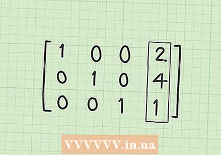11. Search for the solution matrix. At this point, if all went well, you would have the three rows R1 = [1,0,0,2], R2 = [0,1,0,4] and R3 = [0,0,1,1] have to have. Note that if you write this in the block matrix form with the rows one above the other, you have diagonal 1's with 0's further, and your solutions are in the fourth column. The solution matrix should look like this:
    • 1 0 0 2
    • 0 1 0 4
    • 0 0 1 1
12. Understanding your solution. After converting the linear equations to a matrix, you put the x coefficients in the first column, the y coefficients in the second column, the z coefficients in the third column. If you want to rewrite the matrix to equations again, these three lines of the matrix actually mean the three equations 1x + 0y + 0z = 2, 0x + 1y + 0z = 4, and 0x + 0y + 1z = 1. Since we can cross out the 0 terms and not have to write the 1 coefficients, these three equations simplify to the solution, x = 2, y = 4, and z = 1. This is the solution to your system of linear equations.

Part 4 of 4: Checking your solution

1. Include the solutions in each variable in each equation. It is always a good idea to check that your solution is actually correct. You do this by testing your results in the original equations.
   • The original equations for this problem were: 3x + y-z = 9, 2x-2y + z = -3, and x + y + z = 7. When you replace the variables with their values ​​you found, you get 3 * 2 + 4-1 = 9, 2 * 2-2 * 4 + 1 = -3, and 2 + 4 + 1 = 7 .
2. Simplify any comparison. Perform the operations in each equation according to the basic rules of the operations. The first equation simplifies to 6 + 4-1 = 9, or 9 = 9. The second equation can be simplified to 4-8 + 1 = -3, or -3 = -3. The last equation is simply 7 = 7.
   • Since any equation simplifies to a true math statement, your solutions are correct. If any of the solutions are incorrect, check your work again and look for any errors. Some common errors occur when getting rid of minus signs along the way or confusing the multiplication and addition of fractions.
3. Write out your final solutions. For this given problem, the final solution is x = 2, y = 4 and z = 1.

Tips

• If your equation system is very complex, with many variables, you may be able to use a graphing calculator instead of doing the work by hand. For information about this, you can also consult wikiHow.