Content

• Steps

In this article, you will learn how to use a custom formula in the Conditional Formatting menu to select cells with duplicate values.

Steps

1. 1 Open the Google Sheets page in a browser. Enter sheets.google.com in the address bar and press on your keyboard ↵ Enter or ⏎ Return.
2. 2 Click on the table you want to change. Find the one to which you want to apply the filter in the list of saved tables and open it.
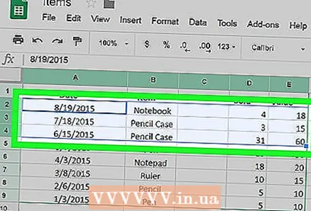3. 3 Select the cells you want to filter. Click on a cell and move the mouse cursor to select adjacent cells.
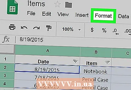4. 4 Click on the tab Format in the tab bar at the top of the sheet. After that, a drop-down menu will appear on the screen.
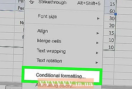5. 5 Select the item in the menu Conditional formatting. After that, a sidebar will appear on the right side of the screen.
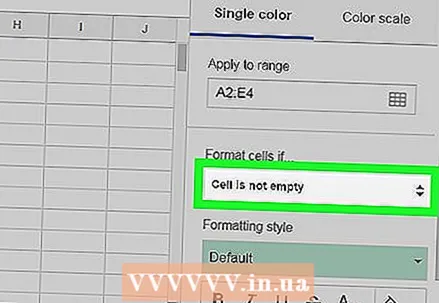6. 6 Click on the drop-down menu under the phrase "Format cells if ...". After that, a list of filters that can be applied to the sheet will appear.
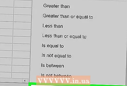7. 7 Select from the drop-down menu item Your formula. With this option, you can manually enter a formula for the filter.
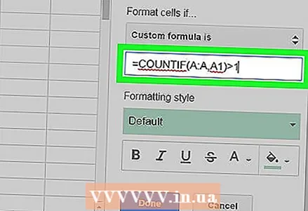8. 8 Enter = COUNTIF (A: A, A1)> 1 in the Value or Formula box. This formula will select all duplicate cells in the selected range.
   • If the range of cells you want to edit is in some other column and not in column A, change A: A and A1 to indicate the desired column.
   • For example, if you are editing cells in column D, your formula will look like this: = COUNTIF (D: D, D1)> 1.
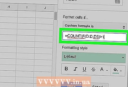9. 9 Change A1 in the formula to the first cell in the selected range. This part in the formula points to the first cell in the selected data range.
   • For example, if the first cell in a range is D5, your formula will look like this: = COUNTIF (D: D, D5)> 1.
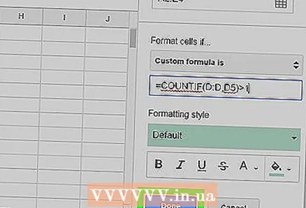10. 10 Click on the green button Readyto apply the formula and select all duplicate cells in the selected range.