Content

• Steps
• Advice

Although Excel is not graphic-oriented, there are many different ways for you to create a timeline. If you use Excel 2013 or later, you can create an automatic timeline from a given table. On older versions, you'll have to rely on SmartArt, built-in templates, or simply sort spreadsheet cells.

Steps

Method 1 of 3: Use SmartArt (Excel 2007 or later)

1. 

   Create a new spreadsheet. SmartArt creates a graphic layout for you to add data. This feature does not automatically fill in your existing data, so you need to create a new spreadsheet for the timeline.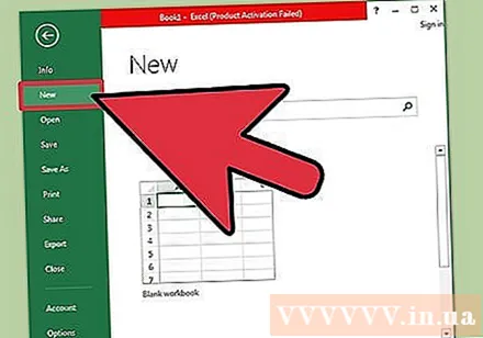

2. 

   
   
   Open the SmartArt menu. Depending on your version of Excel, you can click the SmartArt tab in the ribbon menu, or click the Insert tab and then click SmartArt. This option is available in Excel 2007 and later.

3. 

   Select the timeline from the Process submenu. Click Process in the Insert Smart Art Graphic group in the SmartArt ribbon menu. In the drop-down menu that appears, select Basic Timeline (the arrow points right).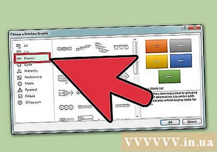
   • You can modify other Process graphics to make your timeline. To see the name of each graphic, hover the mouse pointer over the icon and wait until the text appears.

4. 

   
   
   Add more events. By default, you only have a handful of events available. If you want to add events, you need to select a timeline. The Text Pane text pane will appear on the left side of the graphic. Click the + sign at the top of the text frame to add a new event to the timeline.
   • To zoom in on the timeline without adding new events, click the timeline to display a frame border. Then, click and drag the left or right edge of the frame outwards.

5. 

   
   
   Timeline editing. Enter the data in the Text Pane box to add items. You can also copy and paste data into a timeline for Excel to sort itself. Usually each column of data is an independent timeline item. advertisement

Method 2 of 3: Use Pivot Table Analysis (Excel 2013 or later)

1. 

   Open spreadsheet yes summary or pivot table. To create an automatic timeline, your data must be organized into a pivot table. You will need a pivot table analyze menu, which is featured in Excel 2013.

2. 

   Click anywhere in the pivot table. The "PIVOT TABLE TOOLS" (pivot table tool) will open in the top ribbon.

3. 

   Click “Analyze”. A ribbon with data management options in the table appears.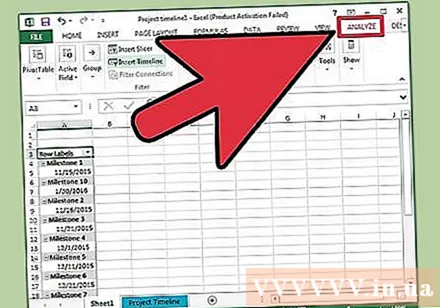

4. 

   Click “Insert Timeline”. A dialog box will pop up with fields corresponding to the date format. Note that if you enter a date in text, it will not be recognized.

5. 

   Select the Applicable field and click OK. A new pane that allows you to navigate through the timeline will appear.

6. 

   Choose how the data will be filtered. Depending on what information is available, you can choose how the data is filtered (by month, year or quarter).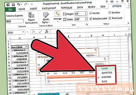

7. 

   Analyze monthly data. When you click a month in the Timeline Control Box, the pivot table will only display data for that particular month.

8. 

   Expand the selection. You can widen the selection by clicking and dragging the sides of the sliders. advertisement

Method 3 of 3: use a basic spreadsheet (on all versions)

1. 

   Consider downloading templates. Although not required, the template will save you time with predefined timeline structures. You can check that you have a timeline template by browsing the options in File → New or File → New from Template. Or you can search online for user-created timeline templates. If you don't want to use a template, proceed to the next step.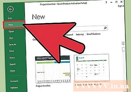
   • If the timeline is used to track the progress of a project with multiple branches, you should consider looking for a "Gantt chart" template.

2. 

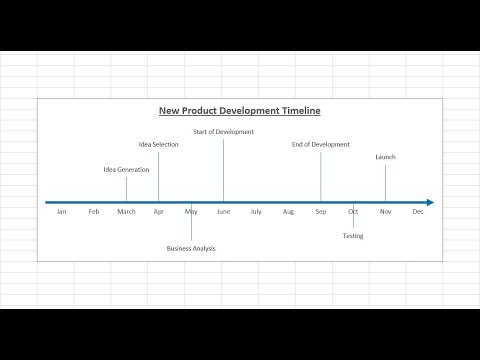
   Start your own timeline from regular cells. You can set up a baseline timeline using a regular blank spreadsheet. Enter the dates of the timeline in a row, separated by blank cells in proportion to the time interval between them.

3. 

   Write the timeline entries. In the box directly above or below each date, describe the event that happened on that day. Don't worry if the data doesn't look good.
   • Adjust descriptions above and below the date to create the most legible timeline.

4. 

   Tilt the descriptions. Select the cell containing your description. Click the Home tab in the ribbon menu, then find the Orientation button below the Alignment options group. (On some versions, the Orientation button is an abc.) Click this button and choose one of the italic options. Once the text has been rotated properly, the descriptions will fit into the timeline.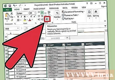
   • In Excel 2003 and earlier, you must right-click the selected cells. Select Format Cells, then click the Alignment tab. Enter the number of degrees you want the text to rotate, and click OK.
   advertisement

Advice

• If you are still not satisfied with these options, then PowerPoint gives you more graphics options.