Content

• Steps
• Advice

Microsoft Office Excel offers a variety of features for customizing tables and charts that contain important information. The program also provides efficient ways to combine and aggregate data from multiple files and worksheets. Common methods for consolidation in Excel include merging by location, by category, using the program's formula or Pivot Table feature. Let's learn how to merge in Excel so that your information shows up in the master worksheet and can be referenced whenever you need to make a report.

Steps

Method 1 of 4: Merge by location on Excel worksheet

1. 

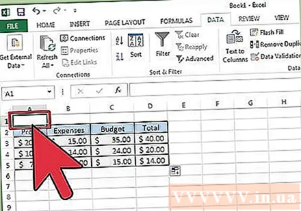
   The data in each worksheet needs to be displayed as a list. Make sure you have deleted all blank columns and rows with the same information label.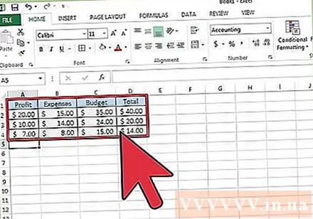
   • Add and arrange each range of columns to split worksheets. Note: The ranges should not be added to the main worksheet that you plan to use for consolidation.
   • Highlight and name each range by selecting the Formulas tab, clicking the down arrow next to the Define Name option, and selecting Define Name (this may differ depending on the Exel version). Then, enter a name for the range in the Name field.

2. 

   
   
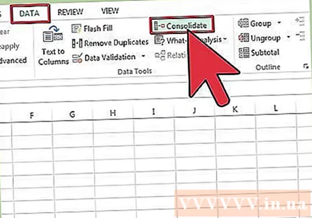
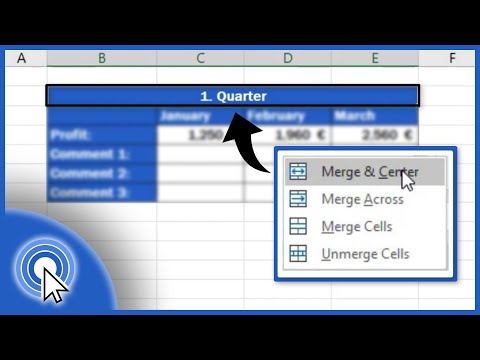
   Prepare to merge Excel data. Click the upper left cell where you want to place the post-merged data on the main worksheet.
   • Go to the Data tab on the main worksheet, and then select the Data Tools tool group. Select Consolidate.
   • Access the summary function summary feature in the Function pane to set data consolidation.

3. 

   
   
   Enter the range name in the Summary Function feature. Click Add to start the merging process.

4. 

   Update merged data. Select Create Links for the Source Data box if you want to automatically update the data source. Leave this box blank if you want to update the data after manually merging. advertisement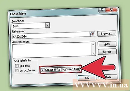

Method 2 of 4: Determine the item to merge Excel data

1. 

   
   
   Repeat the steps at the beginning to set up data in list format. In the main worksheet, you click in the upper left cell where you want to place the data after merging.

2. 

   Go to Data Tools Group. Find the Data tab, then click Consolidate. Use the summary function in the Function pane to set up data consolidation. Give each range a name and then click Add to complete the merging. Then, repeat the process to update the merged data as described above. advertisement

Method 3 of 4: Use a formula to consolidate Excel data

1. 

   Start with the main Excel worksheet. Type or copy the labels of rows and columns that you want to use to consolidate the Excel data.

2. 

   Select the cell where you want to merge the results. On each worksheet, enter the formula that references the cells to merge. In the first cell where you want to include the information, enter a formula similar to this: = SUM (Department A! B2, Department B! D4, Department C! F8). To consolidate all Excel data from all cells, you enter the formula: = SUM (Department A: Department C! F8)

Method 4 of 4: Access the PivotTable feature

1. 

   Create a PivotTable report. This feature allows you to consolidate Excel data from multiple ranges with the ability to reorder items as needed.
   • Press Alt + D + P to open the PivotTable and PivotChart wizard. Select Multiple Consolidation Ranges, then click Next.
   • Select the command “I Will Create the Page Fields” and click Next.
   • Go to the Collapse Dialog dialog box to hide the dialog box on the worksheet. On the worksheet, you select the cell range> Expand Dialog> Add. Under the page field option, enter the number 0 and click Next.
   • Select a location on the worksheet to create the PivotTable report, and then click Finish.
   advertisement

Advice

• With the PivotTable option, you can also use the wizard to consolidate data against an Excel worksheet that has only one page, multiple pages, or no data fields.