Content

• To step
• Method 1 of 2: Add data
• Method 2 of 2: Create a chart
• Tips

In this article, you will learn how to display data in Excel in a more visual way, using a bar chart.

To step

Method 1 of 2: Add data

1. Open Microsoft Excel. Click on the symbol with the white letter "X" against a green background.
   • If you want to create a chart from existing data, open the excel file containing the data by clicking it twice and move on to the next method.
2. Click Blank Worksheet (on a PC) or Worksheet in Excel (on a Mac). You can find this option at the top left of the preview window.
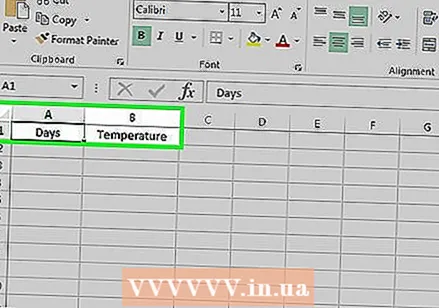3. Add titles to the X and Y axis of the chart. To do this, click on the cell A1 (for the X axis) and type in a designation. Then do the same for the cell B1 (for the Y axis).
   • In a graph showing the temperature of all days of a given week, you would be in cell A1 for example can put "Days" and put in a cell B1 'Temperature'.
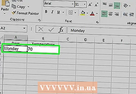4. Enter the data for the X and Y axes. To do this, enter a number or a word in the column of the cell a or B. to apply it to the X or Y axis respectively.
   • For example, if you have "Monday" in cell A2 type and "22" in field B2, that may indicate that it was 22 degrees on Monday.
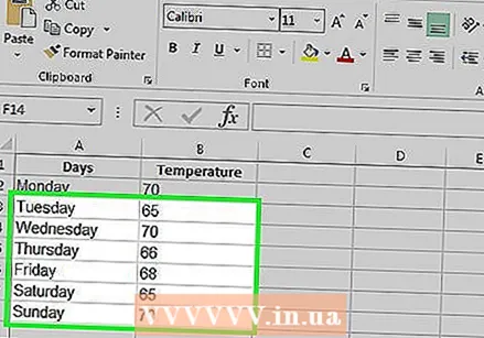5. Enter the other details. Once you have entered all the details, you can create a bar chart based on the information.

Method 2 of 2: Create a chart

1. Select all data. To do this, click on cell A1, please ⇧ Shift and then click the bottom value in column B.. This way you select all data.
   • If you are using different letters and numbers and the like in the columns of your chart, remember that you can just click the top left cell and then click the bottom right cell while at the same time ⇧ Shift pressed.
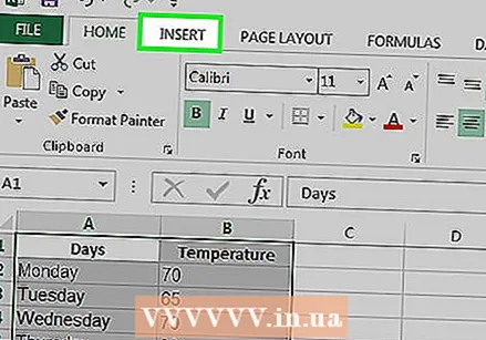2. Click the Insert tab. You can find it at the top of the Excel window, just to the right of the Home tab.
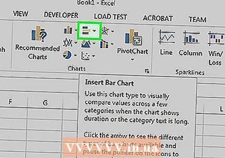3. Click on the "Bar Graph" icon. You can find it in the "Charts" group on the right under the tab Insert; it looks like three vertical bars in a row.
4. Click on one of the different types of bar charts. Exactly which models you can choose from depends on the operating system of your PC and whether you are using the paid version of Excel, but some common options are:
   • 2-D Column - Displays your data in the form of simple vertical bars.
   • 3-D Column - A presentation in three-dimensional, vertical bars.
   • 2-D Bar - Display in the form of a simple graph with horizontal instead of vertical bars.
   • 3-D Bar - Display in three-dimensional, horizontal bars.
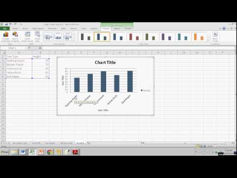
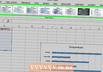5. Customize the look of your chart. Once you've chosen a layout for your chart, you can use the "Design" section near the very top of the Excel window to choose a different design, change the colors, or choose a completely different chart type.
   • The "Design" window only appears when your chart is selected. Click on the graph to select it.
   • You can also click on the chart title to select it and then enter a new name. Usually the title is at the top of the chart window.

Tips

• You can copy and paste charts into other Office programs such as Word or PowerPoint.
• If your graph has swapped the x and y axes of your table, go to the "Design" tab and select "Swap Row / Column" to solve the problem.