Content

• To step
• Method 1 of 2: Using Microsoft Excel
• Method 2 of 2: Using Google Sheets
• Tips
• Warnings

This wikiHow teaches you how to use spreadsheet data to create a chart in Microsoft Excel or Google Sheets.

To step

Method 1 of 2: Using Microsoft Excel

1. Open the Excel program. This resembles a white "E" on a green background.
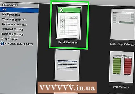2. Click Blank Workbook. This option can be found in the top left of the template window.
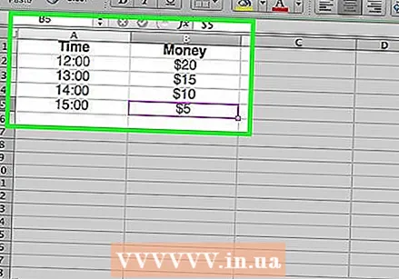3. Enter your information in a spreadsheet. For example, a graph showing expenses per day, where "X" is the time of the day and "Y" is an amount of money:
   • A1 stands for time "Time".
   • B1 stands for "Money".
   • A2 and down then displays different times of the day (such as "12:00" in A2, "13:00" in A3, etc.).
   • B2 and down then represents the decrease in money amounts corresponding to the time in column A ('€ 20' in B2 means that one has 20 euros at 12 noon, '€ 15' in B3 means that one has 15 euros to one hour, etc.).
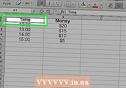4. Click on the top left cell. If you follow the template above, this will be cell A1. This selects the cell.
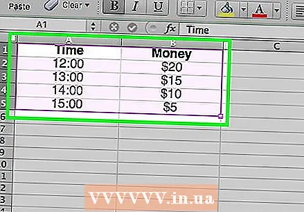5. Keep ⇧ Shift and click on the cell at the bottom right of your data. This action selects all data.
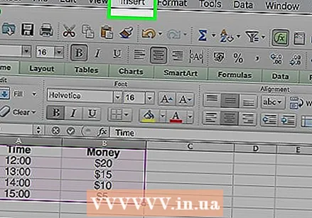6. Click the Insert tab. You will see this option in the green area at the top of the Excel window, to the right of the Starttab.
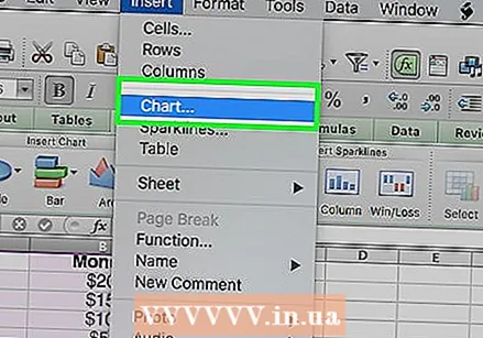7. Click on Charts. This option can be found in the middle of the group of options at the top of the window.
8. Click on a chart option. You can choose from a list of recommended charts based on your data, or click the All chartstab at the top of the window to choose one of the many chart types in Excel.
9. Click OK. You can see this button at the bottom right of the window Insert chart. This will create a graph of your selected data in the format of your choice.
   • You can choose to change the title of the chart by clicking on it and entering a new title.

Method 2 of 2: Using Google Sheets

1. Open the Google Sheets web page.
2. Click Go to Google Sheets. This is the blue button in the center of the page. This will open a new page for selecting a Google Sheets template.
   • If you are not yet logged into Google, enter your email address and click Next one, enter your password and click Next one to proceed to.
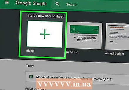3. Click on Empty. These can be found on the left side of the list of options at the top of the page.
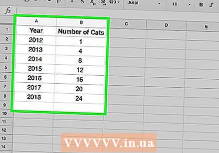4. Enter your details in the spreadsheet. Suppose you have a graph showing the number of cats needed within a certain number of years, where "X" is the year and "Y" is the number of cats:
   • A1 is "Year".
   • B1 is "The number of cats".
   • A2 and further down has different assignments for Year (eg "Year1" or "2012" in A2, "Year2" or "2013" in A3, etc.).
   • B2 and further down may have an increasing number of cats as given, corresponding to the time in column A (e.g., '1' in B2 means one had a cat in 2012, '4' in B3 means one had four cats in 2013, etc.) .
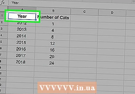5. Click on the top left cell. If you followed the example above, this will become cell A1. This selects the cell.
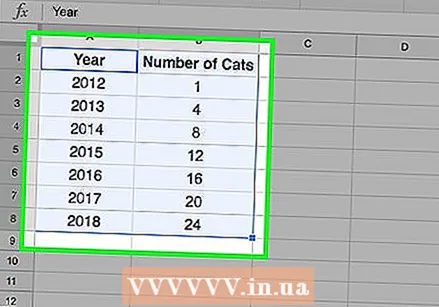6. Keep ⇧ Shift and click the bottom cell of your data. This action ensures that all your data is selected.
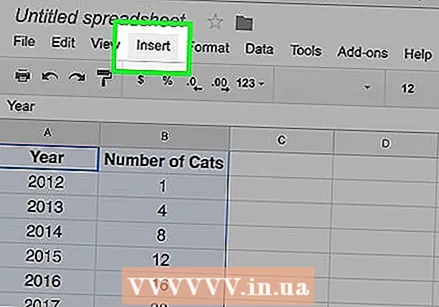7. Click on Insert. This is an entry in the row of options at the top of the page.
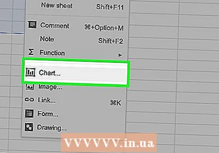8. Click on Chart. This option can be found in the middle of the drop-down menu Insert.
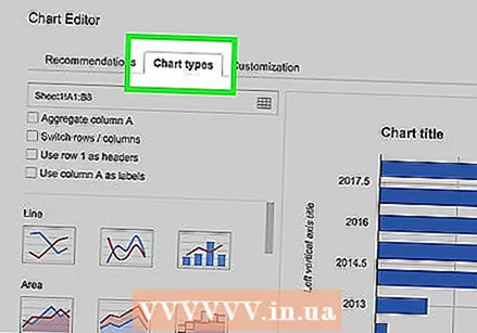9. Click on a chart option. You can choose from a list of recommended charts based on your data, or click the tab Chart type on the right side of the tab Diagrams at the top of the window to view all Google Sheets chart templates.
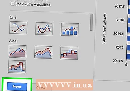10. Click on Insert. You can see this in the lower left corner of the Diagram window. This will create a chart based on your selected data and place it in your Google Spreadsheet.
    • You can click on the chart and drag it anywhere on the page.

Tips

• Google Sheets automatically saves your work.

Warnings

• If you use Excel, don't forget to save your work!