Content

• To step
• Part 1 of 3: Creating the pivot table
• Part 2 of 3: Configuring the pivot table
• Part 3 of 3: Using the pivot table
• Tips
• Warnings

Pivot tables are interactive tables that allow users to group large amounts of data and summarize them in summary tables for easy reporting and analysis. They allow you to sort, count and display data totals and are available in a variety of spreadsheet programs. In Excel you can easily create pivot tables by dragging relevant information into the appropriate boxes. You can then filter and sort your data to discover patterns and trends.

To step

Part 1 of 3: Creating the pivot table

1. Open the spreadsheet you want to make the pivot table of. By means of a pivot table you can visualize the data in a spreadsheet. You can perform calculations without entering formulas or copying cells. You need a spreadsheet with multiple completed cells to create a pivot table.
   • You can also create a pivot table in Excel with an external source, such as Access. You can insert the pivot table in a new Excel spreadsheet.
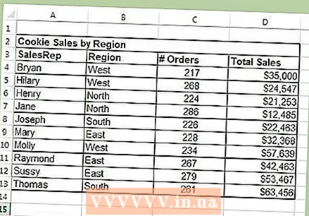2. Make sure your data meets the criteria to create a pivot table. A pivot table is not always the best solution. To take advantage of the properties of a pivot table, your spreadsheet must meet a number of basic conditions:
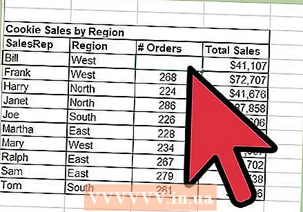
   • The spreadsheet must contain at least one column with equal values. Basically, at least one column must contain data that is always the same. In the example used below, the column "Product Type" has two values: "Table" or "Chair".
   • It must contain numerical information. This is what will be compared and summed in the table. In the example in the next section, the "Sales" column contains numeric data.
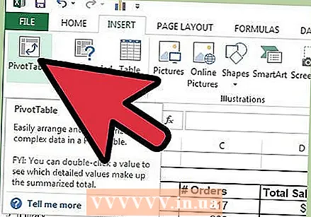3. Start the "Pivot Table" wizard. Click the "Insert" tab at the top of the Excel window. Click the "Pivot Table" button on the left side of the ribbon.
   • If you are using Excel 2003 or older, click on the menu Data and select your PivotTable and PivotChart Report ....
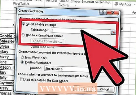4. Select the data you want to use. By default, Excel will select all data on the active worksheet. You can select a specific area of ​​the worksheet by clicking and dragging, or you can type in the range of cells manually.
   • If you are using an external source for the data, click on "Use an external data source", then click Choose connection .... Now choose the location of the connection to the database.
5. Specify a location for your pivot table. After you have selected the range, choose the option "Location" in the same window. Excel will automatically place the table on a new worksheet, so you can easily switch back and forth by clicking the tabs at the bottom of the window. But you can also place the pivot table on the same sheet as your data, that way you can choose which cell it will be placed in.
   • When you are satisfied with your choices, click OK. Your pivot table will now be placed and the appearance of your spreadsheet will change.

Part 2 of 3: Configuring the pivot table

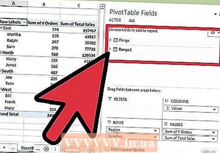
1. Add a row field. Creating a pivot table basically consists of sorting data and columns. What you add determines the structure of the table. Drag a List of Fields (right) to the Row Fields section of the PivotTable to insert information.
   • Suppose your company sells two products: tables and chairs. You have a spreadsheet with the number of (Sales) sold products (Product type) that have been sold in the five stores (Store). You want to see how much of each product has been sold in each store.
   • Drag the Store field from the field list to the Row Fields section in the PivotTable. The list of stores will now appear, each store has its own row.
2. Add a column field. As with rows, you can use columns to sort and display data. In the example above, the Store field has been added to the Row Fields section. To see how much of each type of product has been sold, drag the Product Type field to the column fields section.
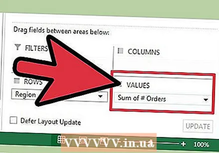3. Add a value field. Now that the organization is ready you can add the data shown in the table. Select and drag the Sales field to the Value Fields section of the PivotTable. You will see that the table shows the sales information for both products in all stores, with a Total column on the right.
   • For the above steps, instead of dragging to the table, you can also drag the fields to the corresponding cells below the list of fields on the right side of the window.
4. Add multiple fields to a section. With a pivot table, you can add multiple fields to each section, giving you precise control over how the data is displayed. We will stay with the above example for a while, now suppose you make different types of tables and chairs. Your spreadsheet indicates whether the item is a table or a chair (Product Type), as well as the exact model of each table or chair sold (Model).
   • Drag the Model field to the column fields section. The columns now show how much has been sold per model and type. You can change the order in which these labels are displayed by clicking the arrow button next to the field in the lower right corner of the window.
5. Change the way the data is displayed. You can change the way the values ​​are displayed by clicking the arrow next to a value in "Values". Select "Value field settings" to change the way the values ​​are calculated. For example, you can display the value as a percentage instead of the total, or you can display the average instead of the sum.
   • You can add the same field multiple times. The example above shows the sales of each store. By adding the "Sales" field again you can change the value settings so that the second field "Sales" is displayed as a percentage of total sales.
6. Learn some ways you can manipulate the values. By changing the way the values ​​are calculated, you have several options to choose from, depending on your needs.
   • Sum - This is the default of all value fields. Excel will sum all values ​​in the selected field.
   • Count - Count the number of cells that contain values ​​in the selected field.
   • Average - This displays the average of all values ​​in the selected field.
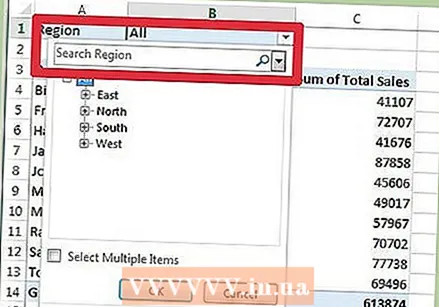7. Add a filter. "Report Filter" contains the fields that allow you to scroll through the summaries of the data, as shown in the pivot table, by filtering out data foundations. They act like filters for the report. For example, if you choose the Store field from your table as your report filter, you can select any store to see individual sales totals, or you can view multiple stores at once.

Part 3 of 3: Using the pivot table

1. Sort and filter your results. One of the most important features of a PivotTable is the ability to sort results and see dynamic reports. Each label can be sorted and filtered by clicking the arrow button next to the label header. You can then sort or filter the list to see only specific data.
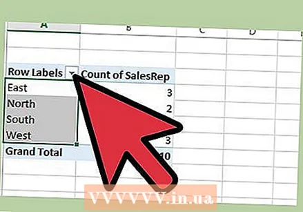2. Update your spreadsheet. Your pivot table will update automatically when you make adjustments to the base spreadsheet. This can be very useful for keeping an eye on the spreadsheets and seeing the changes.
3. Change your pivot table. With pivot tables, it is very easy to change the position and order of fields. Try dragging different fields to different locations to get a pivot table that fits your needs exactly.
   • This is where the name "pivot table" comes from. In a pivot table, you can adjust the direction in which the data is displayed by dragging the data to different locations.
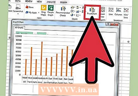4. Create a pivot chart. You can use a pivot chart to view dynamic visual reports. You can create a PivotChart directly from a PivotTable.

Tips

• You have more options for importing data when you click Data> From other sources. You can choose connections from Office database, Excel files, Access databases, text files, web pages or an OLAP cube file. You can then use the data as you are used to in an Excel file.
• Disable "Autofilter" when creating a pivot table. After creating the pivot table you can activate it again.

Warnings

• If you're using data in an existing spreadsheet, make sure the range you select has a unique column name above each column of data.