Content

• Steps

In this article, wikiHow teaches you how to set up and use Microsoft Excel on both Windows and Mac computers.

Steps

Part 1 of 5: Preparation

1. 

   Install Microsoft Office if you don't have one. Microsoft Excel is not distributed as a stand-alone program, but rather as part of the Microsoft Office software package.

2. 

   
   
   Open any Excel document by double-clicking it. This document will open in an Excel window.
   • Skip this step if you want to create and open a new Excel document.

3. 

   Open Excel. Click or double-click the white "X" Excel application icon on a dark blue background.

4. 

   
   
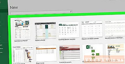
   Select a template if needed. If you want to use an Excel template (such as a budget template), scroll down until you find the template you want to use and click it once to open it in the workbook window.
   • If you just want to open a blank Excel document, click the option Blank (Blank) at the top left of the page and skip to the next step.

5. 

   
   
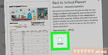
   Press the button Create (Create) to the right of the template name.

6. 

   Wait for the Excel workbook to open. This will take a few seconds. Once the blank page / Excel form appears, you can start importing data into the worksheet. advertisement

Part 2 of 5: Data entry

1. 

   Get familiar with ribbon tags in Excel. On the green "ribbon" at the top of the Excel window are innumerable tabs. It's access to Excel's various tools. The important tags are: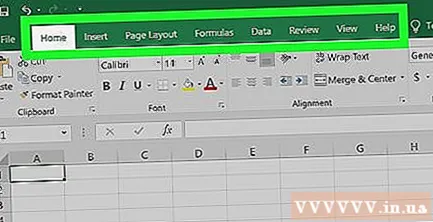
   • Home (Home) - Contains options related to text formatting, changing cell background color and the like.
   • Insert (Insert) - Contains options for tables, charts, graphs, and equations.
   • Page Layout (Page Layout) - Contains options related to aligning, changing page orientation, and choosing a theme.
   • Formulas (Formula) - Contains a function menu and loads of formula options.

2. 

   Consider using the top cells as headings. When adding data to a blank worksheet, you can use the first cell (such as A1, B1, C1, ...) to do column headings. They are very useful in creating tables that require labels.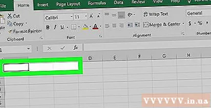

3. 

   Select cell. Click in the cell where you want to import data.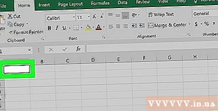
   • In the case of using the budget plan template, for example, you can click on the first empty box to select it.

4. 

   Enter text. Type the text you want to add to the cell.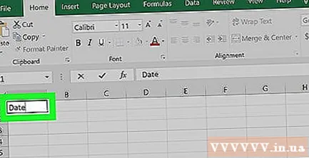

5. 

   Press ↵ Enter to add content to the selected cell and go to the next available cell.

6. 

   Edit your data. To go back and edit the data, click on the cell you want to edit and then make any custom adjustments on the text box above the top row of the spreadsheet.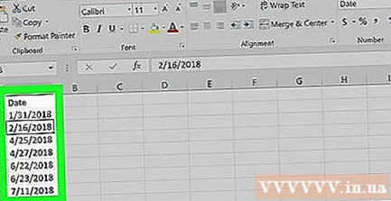

7. 

   Format text if needed. If you want to change the formatting of a cell's contents (such as changing a currency format to a date format), click the tab. Home, in the drop-down box at the top of the "Number" section, and then select the type of format you want to use.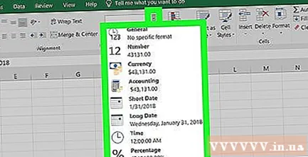
   • You can also use conditional formatting to change the formatting of cells based on certain factors (for example, automatically turns red when the value in the cell is below a certain threshold).
   advertisement

Part 3 of 5: Using formulas

1. 

   Select the cell for your formula. Click in the cell where you want to create the formula.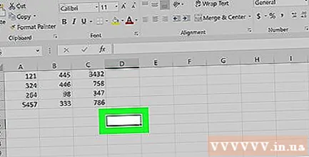

2. 

   Perform simple math operations. You can add, subtract, multiply, and divide cells by the following formulas: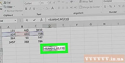
   • Plus - Type = SUM (cell + cell) (For example: = SUM (A3 + B3)) to add the values ​​of two cells together or type = SUM (cell, cell, cell) (For example: = SUM (A2, B2, C2)) to add a range of cells together.
   • Minus - Type = SUM (cell) (For example: = SUM (A3-B3)) to subtract the value of one cell by the value of the other cell.
   • Share - Type = SUM (cell / cell) (For example: = SUM (A6 / C5)) to divide the value of one cell by the value of another cell.
   • Human - Type = SUM (cell * cell) (For example: = SUM (A2 * A7)) to multiply the values ​​of two cells together.

3. 

   Adds the numbers of the column. If you want to add up all the numbers in a column (or part of a column), you can type = SUM (cell: cell) (For example: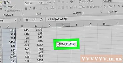 = SUM (A1: A12)) in the cell that you want to use to display the result.

4. 

   Select cells to manipulate with advanced formulas. For a more complex formula, we will use the Insert Function tool. Let's start by clicking in the cell where you want to display the formula.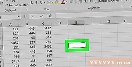

5. 

   Click the card Formulas at the top of the Excel window.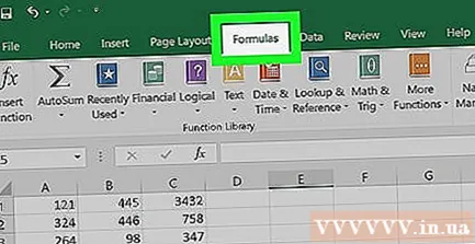

6. 

   Click an option Insert Function on the far left side of the toolbar Formulas. A new window will appear.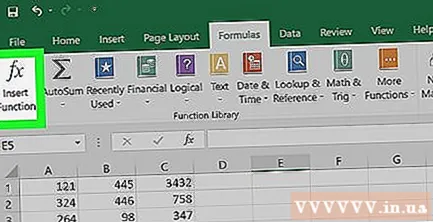

7. 

   Select a function. In the window that opens, click the function you want to use, and then press OK.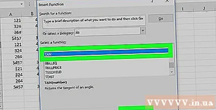
   • For example, to select the tangent formula of a corner, you can scroll and click on the option TAN.

8. 

   Fill out the function form. When prompted, enter the number (or select the cell) for which you want to apply the formula.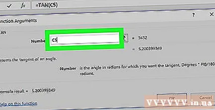
   • For example, when choosing a function TANYou will have to enter the magnitude of the angle for which you want to find the tang.
   • Depending on the function selected, you may have to click through some on-screen instructions.

9. 

   Press ↵ Enter to apply and display the function in the cell you have selected. advertisement

Part 4 of 5: Create a chart

1. 

   Set up the data for your chart. For example, to create a line or column chart, you should create one column of data for the horizontal axis and one column of data for the vertical axis.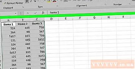
   • Usually the left column is used for the horizontal axis and the column to the right of it is used for the vertical axis.

2. 

   Select data. Click and drag the mouse from the top-left cell down to the bottom-right cell of the data block.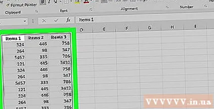

3. 

   On the card Insert (Insert) at the top of the Excel window.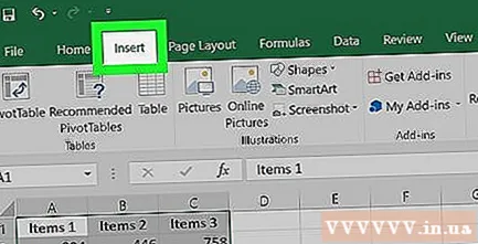

4. 

   Click on the option Recommended Charts (Recommended chart) in the "Charts" section of the toolbar Insert. A window with different chart templates will appear.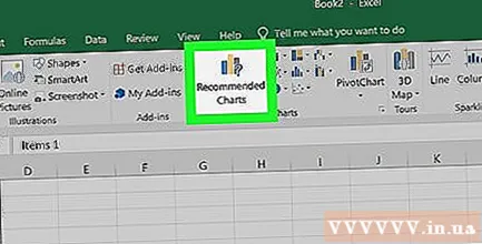

5. 

   Select a chart template. Click on the chart template you want to use.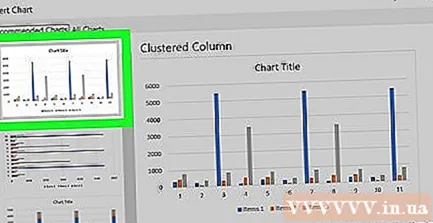

6. 

   Press the button OK at the bottom of the window to create a chart.

7. 

   Edit chart title. Double-click on the title at the top of the chart, delete and replace the current title with your own.

8. 

   Change the titles of the axes. If you want to add axes to your chart, you can go to the "Chart Elements" menu by clicking on the ＋ The green color is just to the right of the selected chart and then make your changes. advertisement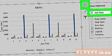

Part 5 of 5: Save an Excel project

1. 

   Click the card File (File) in the upper left side of the Excel (Windows) window or desktop (Mac). A new menu will appear.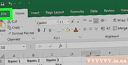

2. 

   Press Save As (Save as). On Windows, this option is located on the left side of the page.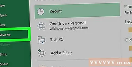
   • For a Mac, this option is in the menu File be dropped.

3. 

   Double-click the option This PC (This computer) is in the middle of the page.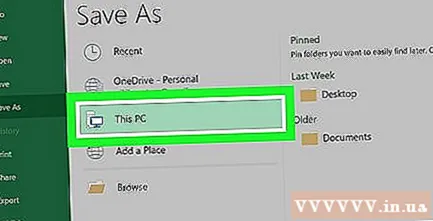
   • With a Mac, that would be On my Mac (On my Mac).

4. 

   Enter your project name. Here, you can use whatever name you want to give your sheet and enter it in the "File name" box - on Windows or "Name" - on a Mac - in the window Save As window.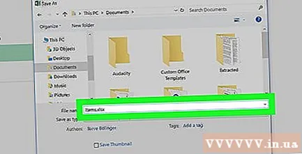

5. 

   Select a save folder. Click the folder where you want to save the worksheet.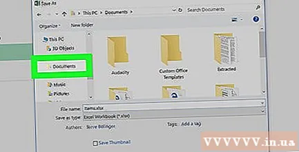
   • On a Mac, you may have to first click the "Where" drop-down box before you can select files.

6. 

   Press Save (Save) at the bottom of the window to save the worksheet to the selected folder under the name you just named.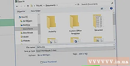

7. 

   Save later edits using the "Save" keyboard shortcut. If you intend to further edit an Excel document, you can press later Ctrl+S (Windows) or ⌘ Command+S (Mac) to save changes without re-entering the Save As window. advertisement